In my last blog post I wrote about the asymptotic equipartition principle. This week I will write about something completely unrelated.

This blog post evolved from a discussion with Brendan O'Connor about science and evidence. The back story is as follows. We were talking about Central Square (Cambridge, MA) and how it is sort of sketchy at night. Brendan mentioned that he had heard some stories about muggings in the area, and I said "Oh yeah, I heard about someone whose place got robbed recently." To which Brendan replied, "Was it in Central?" I told him that I didn't know but that it probably was.

We then got on the topic of whether a crime with an unknown location provided evidence for Central being sketchy. Brendan (who I later learned formalized confirmation bias for his master's thesis) wisely argued that it would depend on the model. I think this is a great point, so in this post I will examine two models that lead to differing conclusions.

I will consider a simplified situation in which there are two areas in town, C and K, and four crimes. The first two crimes occurred C, the third in K, and the fourth may have occurred in either C or K. I will present two alternative statistical models for estimating the "crimeyness" (Brendan's word) of C and K.

The first model treats each crime as an independent draw from a categorical distribution, i.e., each crime occurs in area C with probability (crimeyness) $p$ and in area K with probability $1 - p$. Letting $x_i$ be the location of the $i$th crime, the likelihood function is then

\begin{align*}
&P(x_1 = C, x_2 = C, x_3 = K, x_4 = C \lor x_4 = K \ |\ p)
\\&= P(x_1 = C, x_2 = C, x_3 = K, x_4 = C \ |\ p)
\\&\quad + P(x_1 = C, x_2 = C, x_3 = K, x_4 = K \ |\ p)
\\&= P(x_1 = C, x_2 = C, x_3 = K \ |\ p) ,
\end{align*}

which is just the likelihood of the data without counting the crime in the unobserved location. Thus in this case, that crime adds no evidence for the crimeyness of C.

Roger Grosse inspired the second model I examine here with his insightful comment that, really, the observation of a crime in an unknown location provides evidence for higher crimeyness in all areas.

This model assumes that the number of crimes in C, $n_C$, and the number of crimes in K, $n_K$, have independent Poisson distributions with rate (crimeyness) parameters $r_C$ and $r_K$, respectively.

Ignoring the fourth crime, the likelihood function would be

$P(n_C = 2, n_K = 1 \ |\ r_C, r_K) = P(n_C = 2 \ |\ r_C ) P(n_K = 1 \ |\ r_K),$

which looks like:

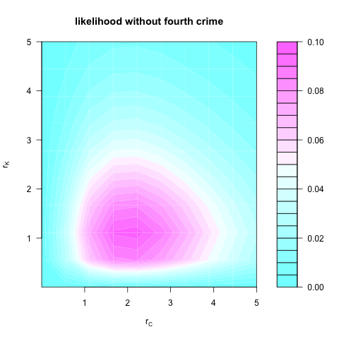
However, including the fourth crime gives the likelihood

\begin{align*}
&P(2 \leq n_C \leq 3, 1 \leq n_K \leq 2, n_C + n_K = 4 \ |\ r_C, r_K)
\\&= P(n_C = 3, n_K = 1 \ |\ r_C, r_K)
\\&\quad + P(n_C = 2, n_K = 2 \ |\ r_C, r_K)
\\&= P(n_C = 3 \ |\ r_C)P(n_K = 1 \ |\ r_K)
\\&\quad + P(n_C = 2 \ |\ r_C)P(n_K = 2 \ |\ r_K),
\end{align*}

which looks like:

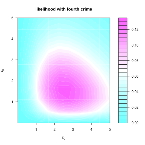
It is clear, then, that including the fourth crime in the second analysis increases the evidence for high crimeyness in both C and K. Thus, as Brendan suggested, whether the crime in the unknown location adds to the evidence of crimeyness depends on the model you use.

Moral of the story: Don't go to Central.

Homework: Is there a model under which the fourth crime provides evidence for higher crimeyness in C but not for higher crimeyness in K?

Also: R code for the plots

Free-association: citogenesis

Disclaimer: Please email me if you find any errors!

I just attended a fun event, Celebrating 100 Years of Markov Chains, at the Institute for Applied Computational Science. There were three talks and they were taped, so hopefully you will be able to find the videos through the IACS website in the near future. Below, I will review some highlights of the first two talks by Brian Hayes and Ryan Adams; I'm skipping the last one because it was more of a review of concepts building up to and surrounding Markov chain Monte Carlo (MCMC).

The first talk was intriguingly called "First Links in the Markov Chain: Poetry and Probability" and was given by Brian Hayes, who also organized today's event and is a Senior Writer at American Scientist magazine. This was a fascinating lecture on the history behind A. A. Markov's work, "An Example of Statistical Investigation of the Text 'Eugene Onegin' Concerning the Connection of Samples in Chains" (January 23, 1913). Hayes began by using the game Monopoly as well as a toy model of weather to introduce Markov chains, (powers of) transition matrices and convergence to stationarity. I especially recommend this part of his talk if you would like to see an excellent example of how to clearly, concisely and concretely present technical material to a general audience. Before diving into some history, Hayes summarized the importance of MCMC in science today by invoking a quote from Persi Diaconis (2009): "To someone working in my part of the world, asking about applications of [MCMC] is a little like asking about applications of the quadratic formula. The results are really used in every aspect of scientific inquiry."

Hayes's history lesson began with Peter the Great's founding of the Academy of Sciences at St. Petersburg, where the likes of Euler and a couple of Bernoulli brothers worked during the 18th century. These foreigners gave way to more Russians in the 19th century, including Chebyshev, and later his student Markov (1856-1922). Incredibly, Markov's work during the early 20th century on convergence of transition matrices was apparently sparked by an argument for free will by Nekrasov, a theologian-turned-mathematician.

The connection between Markov chains and poetry comes through Markov's analysis of Alexander Pushkin's "Eugene Onegin", described by Hayes as "the Russian anthem poem that schoolchildren memorize" and highly recommended by him. Markov took the poem's first 70 stanzas (20,000 characters), removed punctuation and white spaces, counted (!) pairs of characters and calculated their moments. This analysis quantitatively demonstrated a strong tendency to alternate vowels and consonants, which makes sense when you think about pronunciation.

I've left out a lot of historical, political and dramatic details from Hayes's talk -- including the connection to Shannon -- so I hope you have a chance to enjoy a video of his lecture!

Next, Ryan Adams gave a broad overview of how graphical models arise from Markovian concepts, entitled, "From Markov to Pearl: Conditional Independence as a Driving Principle for Probabilistic Modeling". His talk includes lots of recent examples and references; here, I'd like to summarize the topics covered because I think a lot of people will enjoy this talk as a useful introduction to graphical models.

Adams begins with joint probability distributions and their connection to conditional probability distributions through Bayes's Theorem -- he uses a great little computer vision example concerning a photograph of cows and the question, What is in the foreground? Next, he considers two extreme models of (word) sequences to motivate Markov chains: the full joint distribution is really complicated, while the fully factored distribution loses a lot of information. Assuming that each word depends only on the preceding word -- as Markov did with sequences of letters -- yields a model that is only quadratic in the size of the vocabulary.

This Markov property, sometimes referred to as "memorylessness", is a particular case of conditional independence that we can represent through probabilistic graphical models. In these graphs, vertices represent random variables and edges represent conditional distributions; importantly, they aren't restricted to chains but can be any directed acyclic graph. (The lecture slides have lots of useful pictures!) Adams goes over different kinds of information flow in these graphs and covers undirected graphical models (also called Markov random fields) and factor graph models.

A major point that Adams makes is that in addition to the conceptual benefits of graphical models, they also lead to great computational advantages. In particular, the graph -- which recall specifies information flow -- enables inference via efficient message passing algorithms composed of local computations that can be asynchronously updated in parallel. Adams provides a clear example of how to use message passing to compute a marginal distribution.
Efficient online changepoint detection -- important in many applications such as manufacturing and robotics -- exemplifies the power of combining graphical models and belief propagation (Adams and MacKay, 2007) and can be implemented in "a few lines of MATLAB". Adams also mentions loopy belief propagation and makes connections to error correcting codes and data clustering.

Finally, Adams turned to MCMC for graphical models, noting that it can be made efficient through local updates -- basically, you look at your neighbors to do a Gibbs sampling update. Depending on graph's structure, you can try to find colorings that lead to efficient parallel updates; one example is a Restricted Boltzmann machine (RBM), which has bipartite structure.

In the spirit of Ryan's most recent post, I will discuss a fundamental snippet from numerical linear algebra that facilitates computation for the same price of not facilitating it. In our everyday lives, we often come across theoretical expressions that involve matrix inverses stapled to vectors, such as $\Omega^{-1}\mathbf{x}$ with $\Omega\in\mathbb{R}^{n\times n}, \mathbf{x}\in\mathbb{R}^n$. When we proceed to code this up, it is very tempting to first compute $\Omega^{-1}$. Resist doing this! There are several points for why there is no point to actually find an explicit, tangible inverse.

To start off, solving the system $\Omega\mathbf{y}=\mathbf{x}$ for $\mathbf{y}$---using, for example, LU decomposition---is faster and more numerically stable than inverting $\Omega$. Moreover, the real world often bestows us with sparse matrices. The speed of solution of our linear system increases with this sparsity, as it expedites manipulations such as multiplication. Matrix inverses, on the other hand, tend to be dense, and as such do not enjoy these privileges.

Secondly, as the dimension $n$ gets large, our available memory starts to become an issue. Storing the inverse $\Omega^{-1}$ in its full $\mathcal{O}(n^2)$ memory requirement glory is not a task for the faint-hearted. We would much rather deal with matrix-vector products of the form $\Omega^{-1}\mathbf{x}$, which consume $\mathcal{O}(n)$ memory. Furthermore, even if we can't store an $n\times n$ matrix in its entirety, in the case of a sparse matrix, there is hope of storing its nonzero elements. However, again, due to its density, we don't have such hope for an inverse.

Alright, so if we need a single matrix-vector product, it might be better to solve a linear system. What if we are now interested in a number of such products? Even now, it's still better (under a reasonable assumption) to solve a linear system. Once the system is solved for the first time via some decomposition, we have in our hands a factorization of $\Omega$. Hence, we now need an order-of-magnitude less operations to form each future product! Thus, we get a good deal if we need to evaluate less than $\mathcal{O}(n)$ such products.

There are several topics I would like to talk about in the future posts, and they generally fall under the category of theoretical (or systems) neuroscience, and sometimes more broadly biological physics. The topics to be discussed include: the problem of invariance in theoretical neuroscience, Schrodinger's take on physics of living matter and other modern thoughts on fundamental principles underlying biology (optimality principle, role of noise, etc), dynamics and computation: are they mutually exclusive concepts?, correlations (correlations in statistical physics, and the role of correlation in an ensemble of neurons), reinforcement learning, and more. I will start with the post on invariance.

The problem of invariance, in computational neuroscience, is commonly thought of as an effort to understand the nature of the brain's cognitive capacity, invariant despite the presence of latent features, which is irrelevant to the task. Researchers in machine learning and computer vision also seem to be interested in the topic, because (among many other reasons) there are a lot of commercial interests in building algorithms which can recognize useful features in a robust manner. As a theoretical neuroscientist, I am interested in the problem of invariance because the phenomenon seems to be present in various modalities, such as vision, audition, somatosensation, and present across different scales. In the hopeful case, understanding the problem of invariance is perhaps linked with something universal in the information processing of the brain.

First, how can we define invariance? As it refers to the invariance in performance, one has to define a task, and then define latent variables which the performance is invariant under. Consider an example where a subject has to discriminate the direction of a motion of a bar along one axis, say x. In other words, the bar presented twice, and the second bar is shifted slightly, and the subject is forced to decide whether the shift was in the left or the right direction. Suppose that the first bar is at position x, and the second bar is at position x+dx or x-dx where dx is much smaller than x. If the choice of x is at random and the subject does not know what x is explicitly, then x is the latent variable. The problem can be made more complicated (and relevant) by introducing other variables such as the thickness/color/contrast of a bar, etc. These problems are simplified versions of a problem where a subject detects the direction of motion of an arbitrary object regardless of the nature of the visual input produced by the object. This is what we do everyday, when we notice the direction of objects that are moving around us, and it is clear that the real brain can do these tasks well regardless of what the objects are, as long as they produce considerable signals in the visual periphery.

Then can we mathematically define invariance with the task above? The naive and simplest answer would be the following: the performance on the task is exactly the same for each latent variable. This is not wrong, but it is too strict of a definition for the theoretical neuroscientists to say something meaningful about the brain. According to this definition, the brain is certainly not invariant, as shown by numerous psychophysics tests. For example, we are better at discriminating between the orientation of bars around the cardinal angles, compared to the oblique angles [1]. The point is not on the exactly same performance per each latent variable. One has to note that when neuroscientists say invariant recognition/discrimination, what they really refer to is a robust performance. There are two ways one can mathematically define this robustness. One way to describe "invariance" is by comparing the performance to a lower bound given by available information (e.g. Cramer-Rao bound given by Fisher information). In this sense, achieving Cramer-Rao optimality for each latent variable will suffice as an invariant performance. Another definition of invariance is by using the notion that physicists like: "extensivity." If a performance of a particular network structure on a task can be described as a function of signal-to-noise ratio of a network output, then does this signal-to-noise ratio grow linearly with the size of a network N (which corresponds to the number of neurons)? If the extensivity of a neural model agrees with that of an optimal decoder, at least we know that the performance of a network is qualitatively the same as an optimal decoder up to a coefficient (even when the performance of a model is not exactly optimal).

The natural question that follows is, what is a candidate principle for reading out information from sensory response, such that the invariant performance is achieved? As it turns out, the presence of nonlinearity is crucial for achieving an invariant performance (linear decoder is proven to fail the invariant bar discrimination task [2]). Then, what kind of nonlinearly is needed for the readout which can achieve an invariant performance? Answering this question is closely related to the role of correlations in population coding. In the next post, I will discuss the issue of correlations in neural decoding.

[1] Girshick, Ahna R., Michael S. Landy, and Eero P. Simoncelli. "Cardinal rules: visual orientation perception reflects knowledge of environmental statistics."Nature neuroscience 14.7 (2011): 926-932.
[2] Seung, H. S., and H. Sompolinsky. "Simple models for reading neuronal population codes." Proceedings of the National Academy of Sciences 90.22 (1993): 10749-10753.

Jeff Miller and Matthew Harrison at Brown (go Bears!) have recently explored the posterior consistency of Dirichlet process mixture (DPM) models, emphasizing one particular drawback.

For setup, say you have some observed data $x_1, ..., x_n$ from a mixture of two normals, such as

$$p(x|\theta) = \frac{1}{2}\mathcal{N}(x|0,1) + \frac{1}{2}\mathcal{N}(x|6,1)$$

In this case, the number of clusters, $s$, is two, and one would imagine that as $n$ grows, the posterior distribution of $s$ would converge to 2, i.e. $p(s=2|x_{1:n}) \rightarrow 1$. However, this is not true if you model the data with a DPM (or more generally, modeling the mixing measure as a Dirichlet process, $Q \sim DP$).

In this note, the authors show that the DPM is inconsistent for the number of clusters in a single Gaussian. In fact, in this case the inconsistency is so severe that $p(s=1 | x) \stackrel{P}{\rightarrow} 0$ as $n \rightarrow \infty$.

So if $Q \sim DP(\alpha, H)$ doesn't lead to convergence on the number of clusters, then what does?  Miller and Harrison bring attention to a viable alternative called the Mixture of Finite Mixtures (MFM).  The mixing measure is generated by:

• $S \sim p(s)$, a pmf on $\{1,2,...\}$
• $\pi | S=s \sim Dirichlet(\alpha_{s1}, ..., \alpha_{ss})$
• $\theta_1, ..., \theta_s | S=s \sim H$
• $Q = \sum_{i=1}^S \pi_i \delta_{\theta_i}$.

This alternative mixing measure generation provides a consistent posterior on the number of clusters.

At the NIPS Workshop on Modern Nonparametric Methods in Machine Learning, Jeff presented his poster, which nicely outlines some of the advantages of the MFM model, as well as analogous reinterpretations of the model. For example, there exists a Chinese restaurant-like process for MFMs that is comparable to the DPM. Furthermore, the stick-breaking construction for MFMs boils down to a Poisson process on the unit interval. The poster also provides some visual intuition behind why the DP tends to overestimate the number of clusters.

So if what's important to you is the number of latent clusters you might be better off using the MFM for posterior inference. It would be interesting to see how reversible jump MCMC or other trans-dimensional model selection methods compare to MFM posterior inference for recovering the number of clusters.

In machine learning, we often want to evaluate how well a model describes a dataset. In an unsupervised setting, we might use one of two criteria:

1. marginal likelihood, or Bayes factor: the probability of the data, with all parameters and latent variables integrated out
2. held-out likelihood, or the probability of held-out test data under the parameters learned on the training set

Both of these criteria can require computing difficult high-dimensional sums or integrals, which I'll refer to here as the partition function. In most cases, it's infeasible to solve these integrals exactly, so we rely on approximation techniques, such as variational inference or sampling.

Often you'll hear claims that such-and-such an algorithm is an unbiased estimator of the partition function. What does this mean in practice, and why do we care?  Our intuitions from other sorts of unbiased estimators can be very misleading here.

Ordinarily, we like unbiased Monte Carlo estimators because we can improve the accuracy by computing more samples. If we have a stochastic estimator $\hat{\theta}$ of some quantity $\theta$ which is unbiased and has finite variance, we can average $N$ samples together and the mean squared error will decrease like $1/N$. Unfortunately, unless we're very careful, Monte Carlo estimators of partition functions generally have infinite variance, or at least such ridiculously large variance that it might as well be infinite. In these cases, it doesn't matter how many samples we compute -- we're not going to get an accurate answer.

For concreteness, let's consider estimating a partition function using importance sampling. Suppose we have an undirected graphical model over variables $x$ with unnormalized distribution $f(x)$, and we want to estimate the partition function $Z = \sum_x f(x)$. The importance sampling estimator draws a sample from some tractable distribution $q(x)$, and then returns the estimate $f(x) / q(x)$. (We could average over multiple samples, but let's just use one for simplicity.) This is an unbiased estimator, because

$${\mathbb E}_{q(x)} \left[ \frac{f(x)}{q(x)} \right] = \sum_x q(x) \frac{f(x)}{q(x)} = \sum_x f(x) = Z.$$

This naive importance sampling estimator is hardly ever used in practice because it usually has extremely large, or infinite, variance. To get a sense for how common a problem this is, consider the following pair of probability distributions:

$$p(x) = 0.999 N(x; 0, 1) + 0.001 N(x; 0, 2)$$

$$q(x) = N(x; 0, 1)$$

Clearly, p and q represent nearly the same distribution. They should be a piece of cake for any reasonable algorithm. However, if we perform importance sampling with p as the target distribution and q as the proposal distribution, the importance weights will have infinite variance. The problem is that even though the tails of both distributions decay very quickly, the importance weights grow faster than the tails decay. In order to guarantee finite variance, you need to worry even about parts of the distribution which are unlikely and should have little impact on the quantity of interest.

Does this mean it's pointless to talk about unbiased estimators of partition functions?  I'd say no -- instead, we should think of them as biased estimators of the log partition function. Partition functions vary over a lot of orders of magnitude, so it's more natural to think of them on a log scale. And when we take the log, the problem of occasionally getting extremely large values disappears.

I'll give two simple arguments why we should view unbiased estimators of partition functions as stochastic lower bounds. First, Markov's inequality says that for any nonnegative random variable $X$, $P(X > aE[X]) < 1/a$. In the case of partition function estimators $\hat{Z}$ (which are usually nonnegative), this implies that $P(\log \hat{Z} > \log Z + b) < e^{-b}$. In other words, overestimates of the true value are exponentially unlikely.

The second reason to view unbiased estimators as lower bounds comes from applying Jensen's inequality:

$$E[\log \hat{Z}] \leq \log E[\hat{Z}] = \log Z.$$

So its expected value is no larger than the true log partition function. In the case of importance sampling, by expanding out the definitions and rearranging terms, we can go even further and determine the bias of the estimator. If q is the proposal distribution and p is the target distribution, the bias (i.e. $\log Z - E[\log \hat{Z}]$) is given by the KL divergence $D(q \| p)$. Interestingly, this is the same bias as we get in variational Bayes, using q as the approximating distribution. I find this a pretty surprising connection, and I haven't seen it explicitly mentioned anywhere.

So if you don't know anything about a partition function estimator other than that it's unbiased, you already know how to think about it: it's like a lower bound on the true value. This is pretty convenient if you're trying to compute the marginal likelihood of your model. You know your model is almost certainly at least as good as your estimator says.

On the other hand, suppose you're trying to estimate held-out likelihood for an undirected graphical model. In that case, we care about the partition function because it appears in the denominator of the likelihood. A lower bound on the partition function, therefore, translates into an upper bound on the likelihood. If your estimator is wrong, it can be arbitrarily optimistic. Basically, you have no way of telling if your awesome results are due to your model being good, or your partition function estimator being bad. For this reason, experiments which measure the likelihood of undirected models are held to a very high standard. It's necessary to do convergence diagnostics, and even then we don't really have any way of being sure the answer is reasonable.

This, in a nutshell, is what you should think of when you hear a partition function estimator is unbiased.

In my previous post I suggested that models of neural computation can be expressed as prior distributions over functional and effective connectivity, and with this common specification we can compare models by their posterior probability given neural recordings. I would like to explore this idea in more detail by first describing functional and effective connectivity and then considering how various models could be expressed in this framework.

Functional and effective connectivity are concepts originating in neuroimaging and spike train analysis. Functional connectivity measures the correlation between neurophysiological events (e.g. spikes on neurons or BOLD signal in fMRI voxels), whereas effective connectivity is a statement about the causal nature of a system. Effective connectivity captures the influence one neurophysiological event has upon another, either directly via a synapse, or indirectly via a polysynaptic pathway or a parallel connection. In my usage, effective connectivity may include deterministic as well as stochastic relationships. Both concepts are in contrast to structural connectivity which captures the physical synapses or fiber tracts within the brain. Of course these concepts are interrelated: functional and effective connectivity are ultimately mediated by structural connectivity, and causal effective connections imply correlational functional connections.

Many models of neural computation are naturally expressed in causal terms so it is natural to consider their implications for effective connectivity. First we must decide upon a neural representation of the model variables. Some models explicitly describe cell types as well as their synaptic interaction with other cells, for example the linear receptive field model of the retina has ON-center/OFF-center retinal ganglion cells which excite/inhibit their neighbors. In this case we can easily determine a distribution over effective connectivity given a distribution over cell types and their spatial locations. Other models are defined at a computational level in terms of abstract variables, but the encoding of these variables into neural firings is undetermined. For example, consider a motor control model which takes input variables corresponding to the length, velocity, and activation of muscles, and computes a coordinated firing of multiple muscles known as a muscle synergy. There are many ways these variables could be encoded – they could be represented by the firing rate of a set of neurons, or perhaps by a population code. In either case, we can treat the role each neuron plays in the representation of length, velocity, etc. as a latent variable and derive a joint distribution over latent variables and effective connectivity. By marginalizing out the latent variables we arrive at the desired distribution over effective connectivity.

We can use such a distribution over functional or effective connectivity as a prior in a Bayesian model of neural recordings. So long as the connectivity is a latent parameter which generates observable data, we can use Bayesian model comparison to evaluate the most likely model given measured data. Several issues still remain. We must have enough data to adequately fit latent parameters of the prior, and it is not clear how to determine this sample complexity or that modern recording techniques will suffice. Furthermore, I have neglected the murky question of how to actually define a functional or effective connectivity distribution, e.g. are pairwise connections sufficient or must we consider tertiary and higher order connectivity? These are practical considerations en route to realizing a principled model comparison framework.

References:

For a nice discussion of functional and effective connectivity and models thereof, see Chapters 19 and 20 of Human Brain Function, 2^nd Edition by Ashburner, Friston, and Penny. Draft available at:  http://www.fil.ion.ucl.ac.uk/spm/doc/books/hbf2/

This post is about a computational trick that everyone should know, but that doesn't tend to be explicitly taught in machine learning courses.  Imagine that we have a set of $N$ values, $\{x_n\}^N_{n=1}$ and we want to compute the quantity

Continuous problems are often simpler to solve than discrete problems. This is true in many optimization problems (for instance, linear programming versus integer linear programming). In the case of Markov chain Monte Carlo (MCMC), sampling continuous distributions has some advantages over sampling discrete distributions due to the availability of gradient information in the continuous case. The paper “Continuous Relaxations for Discrete Hamiltonian Monte Carlo” by Yichuan Zhang, Charles Sutton, Amos Storkey, and Zoubin Ghahramani explores the idea of performing inference in the discrete setting by deriving and sampling a related continuous distribution. Here I describe the approach taken in this paper.

We consider binary Markov random fields, i.e. discrete distributions over binary vectors ${\bf s} = (s_1, \ldots, s_N)$ of the form

Bayesian nonparametrics allow the contruction of statistical models whose complexity is determined by the observed data. This is accomplished by specifying priors over infinite dimensional distributions. The most widely used Bayesian nonparametric priors in machine learning are the Dirichlet process, the beta process and their corresponding marginal processes the Chinese restaurant process and the Indian buffet process respectively. The Dirichlet process provides a prior for the mixing measure of an infinite mixture model and the beta process can be used as a prior for feature popularity in a latent feature model. The hierarchical Dirichlet process (HDP) also appears frequently in machine learning underlying topic models with an infinite number of topics. A main selling point of Bayesian nonparametrics has been that the complexity of the model can grow as more data is observed. While true in theory, current inference algorithms for Bayesian nonparametric models fail to scale to the massive data sets available making the model impractical. In this post I review traditional inference algorithms for Bayesian nonparametric models and discuss a new approach for handling massive data sets using stochastic variational inference.

Inference in Bayesian nonparametric models is often performed with Markov chain Monte Carlo (MCMC). Many different MCMC methods have been developed to sample from the posterior of interest, examples include Gibbs samplers, slice sampling and retrospective sampling. In fully conditionally conjugate Bayesian nonparametric models these MCMC algorithms can be quite efficient for data sets of moderate size. However, these methods do not scale to massive data sets. There does seem to be a growing body of work on parallelizing these algorithms in order to scale to larger data sets which may be a promising direction. Alternatively, sequential Monte Carlo (SMC) algorithms have been developed as scalable inference algorithms.

Variational inference is an optimization-based alternative to MCMC. The posterior distribution of interest is replaced with a distribution that is simpler to work with called the variational distribution. Most variational algorithms in machine learning utilize the so-called mean-field assumption and assume a fully factorized version of the posterior. Variational algorithms have been developed for many common Bayesian nonparametric models including Dirichlet process mixtures, beta process latent feature models and HDP topic models. However, with few exceptions the algorithms use a truncated representation thus losing the benefit of being nonparametric. Traditionally, variational algorithms are used in a batch fashion assuming all data is observed.  The model parameters are optimized using coordinate ascent to make the variational distribution close (in KL divergence) to the true posterior distribution. In this setting updating the model parameters usually involves all of the data which will scale poorly with the number of observations.

Stochastic variational inference has been introduced as a method to perform variational inference for massive or streaming data sets [1]. The algorithm works by updating observation-specific parameters using coordinate ascent as in standard variational inference. When updating global parameters though, stochastic gradient ascent is used, where a noisy version of the gradient is followed to update the current value of the global parameter. As long as the noisy gradient is equal to the true gradient in expectation and we take smaller and smaller steps in the direction of the noisy gradient the algorithm will converge. In [1] a stochastic variational inference algorithm was derived for a truncated HDP topic model, extending the work in [2] which used stochastic variational inference for applying Latent Dirichlet Allocation to massive text corpora.

Recently, stochastic variational inference has been extended for an infinite HDP topic model in [3]. The key insight of the paper was to use an infinite variational distribution while only allowing a finite number of topics to be used. Specifically, fix a number of topics $K$ and let $q(z_{nj} = k)$ be the probability under the variational distribution that word $j$ in document $n$ is assigned to topic $k$. Assume that $q(z_{nj} = k) = 0$ for $k > K$ so that all infinite dimensional measures in the model (global topic proportions and per-document topic proportions) can be represented as $K+1$-dimensional vectors where the extra dimension contains the probability of a new topic. Under this variational distribution a model with $K$ topics is nested in a model with $K+1$ topics, which does not occur in truncated models as extra probability is assigned to the last mass. The fact that models are nested means that we can compare the variational lower-bound for models with different numbers of topics and can safely add or remove topics in the variational framework. In [3] the authors proposed transdimensional split-merge moves to break a topic into two or combine two topics into one. They found that their algorithm converged to better optima of the variational lower-bound than previous variational algorithms and Gibbs sampling. An alternative infinite online variational algorithm was presented in [4] and may be discussed in a future post.

The infinite online variational algorithm for an HDP topic model discussed is a step toward using Bayesian nonparametrics for massive or streaming data. However, there are drawbacks to the current algorithms, in particular the number of observations (documents for a topic model) must be known in advance. This makes the  infinite online variational algorithms of [1] and [3] unable to handle truly infinite data streams. I think this is an exciting area of research with a lot of interesting work to be done, and perhaps soon we will see Bayesian nonparametrics being used in the real world.

[1] Hoffman, M., Blei, D. M., Wang, C., Paisley, J., Stochastic Variational Inference.  arXiv: 1206.7051.
[2] Hoffman, M., Blei, D.M., Bach, F., Online learning for latent Dirichlet allocation.  In NIPS 2010.
[3] Bryant, M., Sudderth, E., Truly Nonparametric Variational Inference for Hierarchical Dirichlet Processes.  In NIPS 2012.
[4] Wang, C., Blei, D. M., Truncation-free stochastic variational inference for Bayesian nonparametric models.  In NIPS 2012.