The Asymptotic Equipartition Property/Principle (AEP) is a well-known result that is likely covered in any introductory information theory class. Nevertheless, when I first learned about it in such a course, I did not appreciate the implications of its general form.  In this post I will review this beautiful, classic result and offer the mental picture I have of its implications. I will frame my discussion in terms of Markov chains with discrete state spaces, but note that the AEP holds even more generally. My treatment will be relatively informal, and I will assume basic familiarity with Markov chains. See the references for more details.

The intuition for the AEP is most clear in the special case of i.i.d. samples. Consider a chain of $N$ samples from a categorical distribution over the states $1,\ldots,S$ described by the probability vector $\vec{p}$. In this case each symbol will appear about $p_s N$ times with high probability, and in particular the joint probability of each chain will be about $p = p_1^{p_1 N}p_2^{p_2 N}\cdots p_S^{p_S N}$. Interestingly, $\log p = N\sum_s p_s \log p_s = -NH,$ where $H$ is the entropy of the sampling distribution. Thus the probability of most trajectories sampled will be close to $2^{-NH}$.

Somewhat surprisingly, the same results holds for general (ergodic, stationary) Markov chains.  In this case the AEP is stated (as in Shannon [1]): The set of possible length $N$ trajectories of a Markov chain $X_1 = x_1, \ldots, X_N = x_N$ can be partitioned into two disjoint groups, one set whose total probability is arbitrarily small as $N$ increases and another whose members each have a probability $p = P(X_1 = x_1, \ldots, X_N = x_N)$ with $\frac{\log p^{-1}}{N} \approx H$. See Cover and Thomas [2] or the AEP wikipedia page for a proof. This result is called the "equipartition" principle because it says that most of the trajectories in the "typical" or likely set will have approximately equal probability, though I should note that MacKay [3] warns about taking this interpretation too literally.

The reason this is interesting is partly because you might think that as the length of a Markov chain grows there would be $S^N$ trajectories each with approximately equal probability. A moment's thought shows this cannot be the case since trajectories consisting mainly of unlikely states will become far less likely. The AEP formalizes this intuition and gives a precise characterization of the number of likely trajectories. At one extreme a chain with zero entropy, which always samples the same state, will have only one trajectory with nonzero probability. At the other extreme a chain that always samples from the uniform distribution over all states will indeed have what one might naively suspect, $S^N$ equally likely trajectories. The AEP nicely characterizes the rest of the spectrum.

The way I currently visualize the AEP is then as kind of a row property of Markov chains.  Imagine laying out all possible trajectories of a length $N$ Markov chain, $X_1, \ldots, X_N$, in an $S^N \times N$ matrix, where each row $i$ is a trajectory with joint probability $P(X_1 = x_{i1}, \ldots, X_N = x_{iN})$. One important column property of this matrix is that the marginal distribution of the states in any arbitrary column $j$, $P(X_j = x) = \sum_{i} P(X_1 = x_{i1}, \ldots, , X_j = x, \ldots, X_N = x_{iN})$, will be the invariant distribution of the Markov chain. The AEP then describes an interesting row property: the probability mass of $P(X_1, \ldots, X_N)$ is concentrated on only $2^{NH}$ of the $S^N$ rows, and each of those rows has approximately equal probability, $2^{-NH}$. The AEP is thus a fascinating and deep result relating the entropy of a Markov chain to not only the joint probability of its trajectories but also the size of the effective support over its possible trajectories.

[1] Claude E. Shannon. "A Mathematical Theory of Communication", Section 7. The Bell System Technical Journal. 1948.
[2] Thomas M. Cover and Joy A. Thomas. Elements of Information Theory, Chapters 3 and 16.8. Second edition. John Wiley & Sons, Inc. 2006.
[3] David J.C. MacKay. Information Theory, Inference, and Learning Algorithms, Section 4.4. Version 7.2. Cambridge University Press. 2005.

One of the questions in the air at NIPS 2012 was, how do we make machine learning algorithms scale to large datasets? There are two main approaches: (1) developing parallelizable ML algorithms and integrating them with large parallel systems and (2) developing more efficient algorithms. More often than not, the latter approach requires some sort of relaxation of an underlying task. Hashing, streaming algorithms and sketching are increasingly employed to achieve efficient approximate algorithms that arise in ML tasks. Below, I highlight a few examples, mostly from NIPS 2012, with several coming from the Big Learning workshop.

Nearest neighbor search (or similarity search) appears in many "meta" ML tasks such as information retrieval and near-duplicate detection. Many approximate approches are based on locality-sensitive hashing (LSH). The basic idea with LSH is to choose a hash function that maps similar items to the same bucket instead of computing some distance between all pairs of items. For example, some natural language processing (NLP) algorithms depend on nearest-neighbor graphs; LSH can be exploited to efficiently produce approximate nearest-neighbor graphs for large text datasets, e.g., Goyal et al. (2012). While LSH has been around for more than a decade, LSH algorithms are still being developed, e.g., Li et al. (2012) use one permutation hashing to compete with (k-permutation) minwise hashing. A recent area of interest has been in learning a good LSH function automatically from a given dataset; Zheng and Yeung (2012) present one such routine designed for multimodal data.

When a dataset is too large to fit in memory, it may be possible to process the data sequentially with only a limited amount of memory. Streaming is precisely this computational model, in which algorithms are allowed a single or small number of passes over the data; an excellent tutorial-style overview is by Muthukrishnan (2003) . Note that a data stream can often be interpreted as a sequence of 'slices' in time or space. Further, a data set may be thought of as streaming along multiple dimensions, e.g., both time and space, or over some arbitrary serialization of data points, e.g., some ordering of the nodes and edges in a large graph. There is active ML research in both applying existing streaming algorithm results and designing new streaming algorithms motivated by ML problems. Examples include an implementation of expectation maximization for a data stream that is discretized into a series of high-frequency batch computations (Hunter et al., 2012) and streaming algorithms for balanced graph partitioning (Stanton, 2012).

A sketch is a compact representation of data, useful for processing large amounts of data or data streams. It is typically lossy and/or focuses on important statistical features of the data (Cormode, 2011). Li et al. (2006) use sketches to construct conditional random samples for sparse data. A sketch is different from a sample; the latter considers only a portion of the entire data, while the former is computed over all the data. For example, the count-min sketch is able to characterize rare events that would be missed by a sample from a long-tailed distribution (Cormode and Muthukrishnan, 2004). Instead of limiting the size of an input dataset to a ML algorithm by sampling, we can design algorithms that work with sketches. For example, Goyal et al. (2012) - already mentioned above for their use of LSH - a count-min sketch to store the approximate counts of words and other entities of interest for an NLP application.

P.S. Special thanks to Zhenming Liu for his very helpful feedback on this post and Michael Mitzenmacher for CS 222, where I developed an appreciation for topics like hashing, streaming and sketching!

Before diving into more technical posts, I want to briefly touch on some basic questions, and the big picture behind unsupervised learning. I also want to do a bit of handwaving on sparsity---a topic that has gotten a lot of attention recently.

Let's say we are given observations $\mathbf{y}_1,\ldots,\mathbf{y}_N\in\mathbb{R}^D$. These points are assumed to contain some underlying structure, which we seek to capture in order to perform tasks such as classification or compression. We can apply our algorithms on the data in their raw form---which carries unidentified redundancy---and hope for the best. However, a more sensible approach would be to first transform (not necessarily bijectively) the data into a different space via an encoder map $\mathbf{f}:\mathbb{R}^D\rightarrow\mathbb{R}^K$, which we choose to "reshuffle" the information to accentuate interesting patterns in the inputs. We call $\mathbf{x}_n=\mathbf{f}(\mathbf{y_n}),n=1,\ldots,N$ representations of the original data, and now apply our analysis to these instead. To start, we can apply a fixed mapping that we hope will reveal such patterns. Alternatively, we can first define criteria---in the form of constraints, or a cost function---for what makes a "good" representation, and optimize over a large class of parametrized maps to find one that best obeys these. Examples of desirable representation properties are linear independence between representation dimensions, or uniform marginalizations. Maps that achieve these can be found via PCA or the probability integral transform, respectively.

Another very interesting representation criterion is sparsity. A sparse representation of a dataset is one for which in each vector $\mathbf{x}_n$, most of the elements are forced to be zero. The select few that are not are meant to reflect distinguishing features of that example. Let's think about this by considering a standard stacked autoencoder, where the encoder map constitutes of repeated compositions of sigmoidal nonlinearities and linear transformations. In this case, no element in the representation vector will be exactly zero, but we can introduce regularization to ensure lots of elements are very close to it. Can we still maintain true sparsity if we relax the requirement that most elements are exactly zero by allowing these elements to be almost zero (i.e, constraining their magnitudes to be less than some small $\varepsilon>0$)?

The answer is, in general, no. A misconception is that sparsity is a variational bound on element magnitudes, but it is a much deeper statement than that. It says that the sparse elements aren't allowed to capture much---or possibly any---information. More specifically, this demands invariance of the input examples as function of perturbations of the sparse elements, or, in other words, flatness of the input space along sparse directions in the representation space, at the training examples. As such, the indistinguishability of the sparse elements gives rise to an information bottleneck, which is exactly what sparsity is about in the first place.

Returning to our autoencoder question, we see that a 0-th order variational bound isn't sufficient. Sure, the "sparse" elements will pushed close to 0 by some regularization, but they will nevertheless carry nontrivial information content! The only difference is that the decimal place will be shifted. There's really nothing special about the number zero: we could've just as well induced sparsity around $\pi$. The decoder of the stacked autoencoder will be able to pick up a complex enough of a map that it will be able to differentiate between distinct values in the sparse regime, and thus undo the pseudo-sparse compression into the epsilon-ball around zero. It's even worse than that: not only the sigmoid nonlinearities don't give us true zeros, these maps are asymptotically flat (that is, from the input space into representation space) as the representation elements gets close to zero! Had our decoder been the inverse of the encoder, we would've gotten exactly the opposite of the flatness property we actually want.

So, which nonlinearities can we instead use to induce true sparsity? Check out the rectifying nonlinearity as a (generally non-invertible) example of such map.

Say you have a set of $n$ $p$-dimensional iid samples $$\{ \textbf x_i \}_{i=1}^n$$ drawn from some unknown continuous distribution that you want to estimate with an undirected graphical model. You can sometimes get away with assuming the $\textbf x_i$'s are drawn from a multivariate normal (MVN), and from there you can use a host of methods for estimating the covariance matrix $\Sigma$, and thus the graph structure $\Omega = \Sigma^{-1}$ (perhaps imposing sparsity constraints for inferring structure in high dimensional data, $n<<p$).

In other cases the Gaussian assumption is too restrictive (e.g. when marginals exhibit multimodal behavior).

One way to augment the expressivity of the MVN while maintaining some of the desirable properties is to assume that some function of the data is MVN. So instead of modeling the $\textbf x_i$'s as MVN, relax the assumption and model a function of the components $f(\textbf x_i) = (f_1(x_1), ..., f_p(x_p))$ as MVN with mean $\mu$ and covariance $\Sigma$. Now the goal is to estimate $f, \mu, \Sigma$, which characterizes the distribution. Distributions of this type are referred to as nonparanormal (or Gaussian copula distribution).

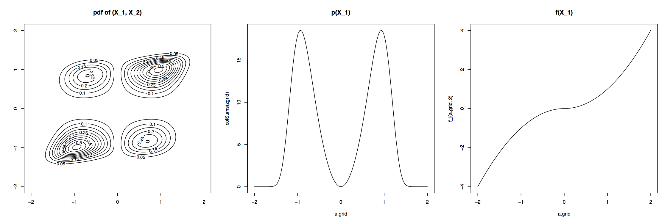
The plots below show an example $NPN$ with $f_j(x_j) = sgn(x_j)|x_j|^{\alpha_j}$.  The plots show the contours for a 2-D $NPN$ distribution, one of the marginals, and one of the transformation functions $f$ (recreated from Lui 2009).

More formally, $X=(X_1, ..., X_p)^T$ has a nonparanormal distribution if there exist a set of functions $\{f_1, ..., f_p\}$ such that $(f_1(X_1), ..., f_p(X_p)) \sim N(\mu, \Sigma)$. This is denoted by $X \sim NPN(\mu, \Sigma, f)$ (Lui 2009).

The resulting density function of the $NPN(\mu, \Sigma, f)$ (assuming the $f$'s are continuous and monotonic) is:
$$ p(x) = \frac{1}{(2\pi)^{p/2}|\Sigma|^{1/2}} \exp \left( -\frac{1}{2}(f(x)-\mu)^T \Sigma^{-1} (f(x) - \mu) \right) \prod_{i=1}^p |f_j'(x_j)| $$

From here, you can derive the important property that if $X\sim NPN(\mu, \Sigma, f)$ is nonparanormal and each $f_i$ is differentiable, then the conditional independence structure of the data is still encoded in the inverse covariance matrix $\Omega = \Sigma^{-1}$.  It also follows that the graph structure (i.e. the inverse covariance zero locations) of the transformed, normal variables is identical to the graph structure of the non normal variables.  This allows you to estimate the graph structure as if the data were normal (with some care).

Now a whole bunch of techniques (graph/structure estimation, inference, etc) can be extended to this richer set of models.  Lui et al 2009 present techniques for estimating undirected graphical models when $n << p$.  A recent paper from NIPS (Elidan and Cario) formalizes belief propagation in a nonparanormal setting.

Another interesting study of inverse covariance and graph structure (on discrete data) is the "No Voodoo Here" (Loh and Wainwright) paper from NIPS this past year.  Though I haven't closely read it, a close examination of the two may shed light on new structure estimation algorithms in high dimensional data.

Often the goal of inference and learning is to use the inferred marginal distributions for prediction or classification purposes. In such scenarios, finding the correct “model structure” or the true “model parameters”, via maximum-likelihood (ML) estimation or (generalized) expectation-maximization (EM), is secondary to the final objective of minimizing a prediction or a classification cost function. Recently, I came across a few interesting papers on learning and inference in graphical models by direct optimization of a cost function of the inferred marginal distributions (or normalized beliefs) [1, 2, 3, 4]:

$$ e = C( outcomes, f(bs); \Theta),$$

where f is a differentiable function that maps the beliefs (bs) to the outcomes/labels of interest, $ \Theta $ is a set of model parameters, and C is a differentiable cost function that penalizes for incorrect classifications or prediction.

The main idea of discriminative learning is to use “back-propagatation” to calculate the gradient of the error e with respect to the marginals and model parameters. In direct analogy to learning in neural networks, one has to keep track of every step of inference (forward pass) and then reverse the operations (reverse mode automatic differentiation) to calculate the error gradient, which will be used for minimization of the classification/prediction error.

I saw one of the first references to this idea in Memisevic (2006) [1] under the so called structured discriminative learning. In Eaton and Ghahramani (2009) [2], error back-propagation with respect to belief-propagation operations was used within a Cutset Conditioning algorithm  (turning a complex graphical model into a simpler one by conditioning on a set of variables) to decide which variables to condition on. Domke [3] and Stoyanov et al. [4], in the context of learning in Markov random fields, showed that discriminative/supervised learning using error back-propagatation can yield better results than likelihood maximization techniques.

In summary, the approach discussed above allows for applying optimization techniques from the neural network literature to learning in some classes of graphical models, and conversely, to use ML and EM-based techniques to initialize equivalent neural network representations of graphical models for supervised training. The latter may resolve some of the traditional issues with initialization and generalization performance of neural networks, and is related to the recent developments in Deep-Learning.

[1] R. Memisevic, "An introduction to structured discriminative learning," Citeseer, Tech. Rep., 2006.
[2] F. Eaton and Z. Ghahramani, "Choosing a variable to clamp: approximate inference using conditioned belief propagation," In Proceedings of AISTATS, vol. 5, pp. 145–152, 2009.
[3] J. Domke, "Beating the likelihood: Marginalization-based parameter learning in graphical models."
[4] Stoyanov, Veselin, Alexander Ropson, and Jason Eisner. "Empirical risk minimization of graphical model parameters given approximate inference, decoding, and model structure." Proceedings of AISTATS. 2011.

The method of moments is a simple idea for estimating the parameters of a model. Suppose the observed data are sampled iid from a distribution $p(x|\theta)$, our goal is to estimate the parameter $\theta$. If we have enough data, we can get very close to the true mean of the distribution, $E[x]$, which is a  function of $\theta$: $E[x]=f_1(\theta)$. We know the form of $f_1$ since we know the form of $p(x|\theta)$.

For simple distributions, knowing just the mean is enough to invert $f_1$ to obtain $\theta$. In general, we need to calculate the higher moments, which are also known functions of $\theta$: $E[x^2] = f_2(\theta), ..., E[x^n]=f_n(\theta)$. We then try to invert the systems of equations $f_1, ..., f_n$ to obtain $\theta$. In practice, we typically only have enough data to accurately estimate the low order ($\leq 3$) moments.

This idea has been used in a series of papers Anima Anandkumar, Daniel Hsu, Sham Kakade, and colleagues to estimate parameters in latent variable models. A very nice introduction of the method is here. Its claim to fame is that if the modeling assumptions are correct and we have enough data, then the method is guaranteed to find the global optimal parameters. This contrasts with popular methods like EM which is often stuck at local optimum.

A particularly cool application is that we can learn all the topics of a Latent Dirichlet Allocation (LDA) model using only the first three moments.  This sounds too good to be true, but a back of the envelope calculation shows that it's actually reasonable. In LDA, each topic is a multinomial distribution over the vocabulary. So say the vocabulary is ~10,000 words and we want to estimate 100 topics, then we have ~ 1 million parameters. The third moments contains all probabilities of the form p(word1, word2, word3), where word1,2,3 can be any words in the vocabulary. Assuming we can estimate the third moments, then we have $~10,000^3=10^{12}$ data points to estimate $10^6$ parameters. Certainly plausible!

The method is quite intuitive. Suppose for simplicity we have an LDA model where each document has exactly one topic. Let $\mu_k$ denote the (true) distribution for topic $k$. The second moment $M_2$ is just the $NxN$ matrix (N=vocab size), where the  $(i,j)$ entry is p(word_i, word_j). This can be written as a sum of outer products, $M_2 = \sum_{k=1}^K \mu_k \mu_k^{T}$. Similarly the third moment is a third order tensor, which generalizes the outer product, $M_3=\sum_{k=1}^{K} \mu_k \bigotimes \mu_k \bigotimes \mu_k$. The key point to notice is that $M_3$ is a rank K tensor, whose eigenvectors are simply $\mu_k$! Once we observe this, the rest of the algorithm comes down to using power iteration methods to recover the tensor eigenvectors, which give us the topic distributions. Very cool.

One basic aim of cognitive neuroscience is to answer questions like 1) what does a neuron or a group of neurons represent, and 2) how is cognitive computation implemented in neuronal hardware?  A common critique is that the field has simply failed to shed light on either of these questions. Our experimental techniques are perhaps too crude: fMRI's temporal resolution is way too slow, EEG and MEG's spatial resolution is far too coarse, electrode recordings miss the forest for the trees. But underlying these criticisms is the assumption that there is some implementation-level description of neural activity that is interpretable at the level of cognition: if only we recorded from a sufficient number of neurons and actually knew what the underlying connectivity looked like, then we could finally figure out what neurons are doing, and what they represent -- whether it's features, or population codes, or prediction error,  or whatever.

Is this a reasonable thing to hope for? Should neurons be interpretable at all? Clearly, no, Marr Level-1-ophiles will argue. After all, you wouldn't hope to learn how a computer works by watching its bits flip, right?

I wonder whether this analogy is fundamentally wrong. What is our assumption about how neurons work that makes it so? One possibility is that we are assuming that changes in the brain (changes in programming) are spatially local and fine-grained: that is, changes occur on the scale of individual neurons. Thus, if these changes can be semantically coherent then that fine gain must carry coherent semantics. In computers, on the other hand, the induced changes are the ones we induce when we interact with them: they are coarse. We write whole programs to change many behavioral elements at once. Therefore, smaller units than those we manipulate need not themselves carry a coherent semantic value.

Does this distinction seem like the right one?

Some of the common complaints I hear about (learning) theoretical work run along the lines of "those bounds are meaningless in practice," "that result doesn't apply to any algorithm someone would actually use," and "you lost me as soon as martingales/Banach spaces/measure-theoretic niceties/... got involved." I don't have a good answer for the latter concern, but a very nice paper by Sasha Rakhlin, Ohad Shamir, and Karthik Sridharan at NIPS this year goes some ways toward address the first two criticisms. Their paper, "Relax and Randomize: From Value to Algorithms," (extended version here) is concerned with transforming non-constructive online regret bounds into useful algorithms. The paper builds off previous statistical learning theory results for worst-case online learning by authors together with Ambuj Tewari. This preprint provides a summary of results for learning from sequential, dependent data. Their results mirror those for the i.i.d. setting, and  include necessary and sufficient conditions for uniform convergence of empirical processes with dependent data; notions of covering numbers, fat-shattering dimension, Rademacher complexity, and other measures of function class complexity in the sequential setting; and a variety of regret bounds based on these quantities.

The essential idea of Rahklin et al.'s approach to statistical learning theory for dependent sequences is to view learning as a 2-player game between the learner and Nature. This hearkens back to a classic way of doing worst-case analysis of online algorithms. In that scenario, the algorithm chooses some strategy $i$ and Nature (a.k.a. the Adversary) chooses some sequence $j$ to give the algorithm. This results in some loss $a_{ij}$ for the algorithm. Forming a (possibly infinite) matrix $A = (a_{ij})$, if the algorithm chooses a strategy according to $p$ (distribution over rows of $A$) and Nature according to $q$ (distribution of columns), then we are interested in the value of the game,

\[ V = \min_p \max_q pAq = \max_q \min_p pAq.\]

Here, the algorithm tries to minimize its loss while Nature tries to maximize the algorithm's loss. The value of the game gives an upper bound for the loss (and hence performance) of the algorithm.

The situation is a little more complicated for online learning. Let $\mathcal F$ be the moves of the learner and $\mathcal X$ be the moves of Nature. For a finite number of rounds $t = 1,\dots, T$, the learner and Nature choose $f_t \in \mathcal F$ and $x_t \in \mathcal X$ and then observe each other's choices. These move pairs are used to define a loss function $\ell : \mathcal F \times \mathcal X \to \mathbb R$. The overall loss for the game is the regret

\[\textbf{Reg}_{T} := \textstyle\sum_{t=1}^{T} \ell(f_{t}, x_{t}) - \inf_{f \in \mathcal F}  \sum_{t=1}^{T} \ell(f, x_{t}).\]

The second term relativizes the loss so that the algorithm is compared to how well you could have done if you had chosen the best possible $f \in \mathcal F$ from the start. Unlike in the algorithms case, the value of the online learning "game" has interleaved min's and max's (well, inf's and sup's), since there are $T$ rounds in the game:

\[\mathcal{V}_T(\mathcal F) = \inf_{p_1 \in \Delta(\mathcal F)} \sup_{x_1 \in \mathcal X} \mathbb E_{f_1 \sim p_1} \cdots  \inf_{p_T \in \Delta(\mathcal F)} \sup_{x_T \in \mathcal X} \mathbb E_{f_T \sim p_T} \textbf{Reg}_T,\]

where $\Delta(\mathcal F)$ is the set of all distributions over $\mathcal F$. In the learning scenario, the expectation plays the role as $pAq$ and Nature's move can be deterministic while still giving the same value.

What Rahklin et al. do is consider relaxations, i.e. upper bounds, to $\mathcal{V}_T(\mathcal F)$ (well, actually the bound a conditional form of $\mathcal{V}_T(\mathcal F)$). These relaxations are chosen to be more manageable to deal with analytically. At the $t$-th stage of the game, instead of finding $p_t$ based on the expression for $\textbf{Reg}_T$, an approximate $p_t$ is calculated. This $p_t$ is the distribution over $\mathcal F$ that minimizes an expression that involves the maximum of the relaxation plus an expected loss term. Since the relaxation can be handled analytically, one now has an actual algorithm for calculating $p_t$, which can be used to make a prediction. The authors derive sometimes improved versions of classic algorithms as well as some new ones. For example, they give  a parameter-free version of exponential weights which optimizes the learning rate in an online manner. Specifically, in round $t$, for each $f \in \mathcal F$

\[ p_t(f) \propto \exp(-\lambda_{t-1}^* \textstyle\sum_{s=1}^{t-1} \ell(f, x_s)) \]

where

\[  \lambda_{t-1}^* = \arg\min_{\lambda > 0} \left\{ \frac{1}{\lambda}  \log \left (\sum_{f \in \mathcal F} \left(- \lambda\textstyle\sum_{s=1}^{t-1} \ell(f, x_s) \right)\right)  + 2\lambda (T - t) \right \} \]

is the optimal learning rate. The relaxation can then be used to bound the regret of the algorithm by $2 \sqrt{2 T \log |\mathcal F|}$. There are many other algorithms discussed, including mirror descent, follow the perturbed leader, and a matrix completion method. I highly recommend checking out the paper for the rest of the details and other examples.

My aim in this introductory post is to provide context for future contributions by sharing my thoughts on the role of computer scientists in the study of brain, particularly in the field of computational neuroscience. For a field with “computation” in the name, it seems that computer scientists are underrepresented. I believe there are significant open questions in neuroscience which are best addressed by those who study the theory of computation, learning, and algorithms, and the systems upon which they are premised.

In my opinion “computational neuroscience” has two definitions: the first, from Marr, is the study of the computational capabilities of the brain, their algorithmic details, and their implementation in neural circuits; the second, stemming from machine learning, is the design and application of computational algorithms, either to solve problems in a biologically-inspired manner, or to aid in the processing and interpretation of neural data. Though quite different, I believe these are complementary and arguably co-dependent endeavors. The forward hypothesis generation advocated by the former seems unlikely to get the details right without the aid of computational and statistical tools for extracting patterns from neural recordings, guiding hypothesis generation, and comparing the evidence for competing models. Likewise, attempts to infer the fundamentals of neural computation from the bottom-up without strong inductive biases appear doomed to wander the vastness of the hypothesis space. How then, can computer scientists contribute to both aspects of computational neuroscience?

Ultimately the brain is a biological computation device and, as such, should fall within the purview of the theory of computation. The brain, like our silicon computers, is also a dynamical system, but when we describe in silico computation we do not discuss attractors and limit cycles (except in the case of infinite loops!). We discuss instructions and variables, the manipulation of symbols given a model of computation. Such abstractions allow us to analyze the complexity of programs. Similarly, I think neural computation should be studied with an appropriate model of computation that enables theoretical analysis and allows us to rule out hypotheses inconsistent with realistic complexity bounds.

For example, the Bayesian brain hypothesis states that the brain is an inference engine, evaluating posterior probabilities of the world given sensory observations. Unfortunately even approximate inference is, in general, NP-hard (w.r.t. Turing machines, though there is little evidence the brain solves NP-hard problems). Of course the brain could be doing variational inference, operating on sufficient statistics, using belief propagation, etc.; such refined algorithmic hypotheses are born of simple complexity arguments. Though I am skeptical of the algorithmic theories put forth thus far, I think the Bayesian brain is an attractive computational hypothesis. Probabilistic programming, which combines the expressiveness of Bayesian networks with deterministic control flow, seems like a natural language for neural computation. How such programs are “compiled” to run on a plausible neural architecture, what instruction set is appropriate for such an architecture, what functions would be expected of a neural “operating system,” and how neural programs are learned and updated through experience, are all questions that computer scientists are particularly suited to address.

In some sense, however, formulating reasonable hypotheses is not the hard part. Choosing among reasonable hypotheses seems to be the challenge. Ideally, we would like to compare the statistical evidence for competing hypotheses given actual data.  Complex models with many parameters and large amounts of data present a computational challenge where, again, computer scientists, particularly machine learning researchers, may contribute. One of my projects has been the creation of a general probabilistic model for spike trains recorded from populations of neurons in which algorithmic hypotheses are expressed as priors on the functional connectivity among the population. A fully-Bayesian inference algorithm enables principled model comparison. This is just a start – not all hypotheses are naturally expressed as functional connectivity priors – but I believe this is ultimately how the comparison of complex models with many parameters must be done.

Of course, it is possible that none of our top-down hypotheses have particularly strong evidence, in which case we would like the data to guide hypothesis generation. This is, essentially, unsupervised machine learning. If the hypothesis class is a space of probabilistic programs, then it is program induction. If the hypothesis class is the space of binary functions, then it is learning Boolean circuits. I’ve expressed my doubts about achieving this in full generality, but I think there is hope in an active-learning paradigm, especially when our inductive biases limit the hypothesis space. Understanding the theoretical limits of such a paradigm would be of interest to the learning theory community, but also has a natural interpretation in the neural setting. Optical tools allow us to manipulate subpopulations of neurons and observe the response of others. A general method for leveraging this white-box access could find broad application in hypothesis testing and generation.

I suspect neural computation is governed by sophisticated programs rather than simple laws, and that the brain is better viewed as a computational machine than as a dynamical system. As we probe further into the workings of the brain the need for a computer science perspective in hypothesis generation and testing, as well as in the interpretation of large and complex datasets, will only become more pressing.

Much of what we do when we analyze data and invent algorithms is think about estimators for unknown quantities, even when we don't directly phrase things this way.  One type of estimator that we commonly encounter is the Monte Carlo estimator, which approximates expectations via the sample mean.  That is, many problems in which we are interested involve a distribution $\pi$ on a space $\mathcal{X}$, where we wish to calculate the expectation of a function $f(x)$: