As the title of the post suggests, this week I will discuss a geometric intuition for Markov's inequality, which for a nonnegative random variable, $X$, states
$$
P(X \geq a) \leq E[X]/a.
$$
This is a simple result in basic probability that still felt surprising every time I used it... until very recently. (Warning: Basic measure theoretic probability lies ahead. These notes look like they provide sufficient background if this post is confusing and you are sufficiently motivated!)

I used to get intuition for Markov's inequality from the fairly intuitive proof (or the equivalent proof with integrals),
\begin{align*}
E[X] &= \sum_x x P(x)
\\
&= \sum_{x < a} x P(x) + \sum_{x \geq a} x P(x)
\\
&\geq \sum_{x \geq a} x P(x)
\\
&\geq \sum_{x \geq a} a P(x)
\\
&= a\sum_{x \geq a} P(x)
\\
&= a P(x \geq a),
\end{align*}

which is all well and good, but I like pictures and don't feel like I have really internalized a concept unless I have a representative picture for it in my mind. The problem is then, what is the picture here? Expectations are averages, so when you look at the value of $E[X]$ it is kind of at the center of the distribution, but how is that related to the probability in the tail of the distribution?

This might be overkill, but in my mind, the key to an intuitive geometric understanding of Markov's inequality relies on a measure theoretic view of probability. What measure theoretic probability gives us in this case is a geometric perspective of expectations, from which Markov's inequality falls out immediately.

Recall that random variables are actually functions. A random variable is defined with respect to a probability triple, $(\Omega, \mathcal{F}, P)$. The function $X\colon \Omega \rightarrow \mathbb{R}$ is a random variable if it is a measurable function in the sense that the preimage $X^{-1}(A) = \{\omega \in \Omega\ |\ X(\omega) \in A\}$ is always measurable, so we can write $P(X \in A) = P(\omega \in X^{-1}(A))$.

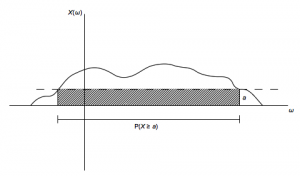
The key is then that $E[X]$ is essentially just the area under the random variable $X$ since $E[X] = \int_\omega X(\omega) dP $. We can then understand Markov's inequality from the following (slightly simplified) picture:
The dashed line is at the height $a$, so the probability that $X$ is greater than $a$ in this case is just the length of the contiguous set of values $\omega$ that map to values of $X(\omega)$ greater than $a$ (the line segment shown in the picture). The area of the shaded box is thus $a P(X \geq a)$, which is clearly less than the entire area under $X(\omega)$. Hence $a P(X \geq a) \leq E[X]$ as desired.

When implementing algorithms for inference and learning with probabilistic models, it commonly comes up that one needs to sample from a discrete distribution. That is, from a multinomial distribution with parameter $\boldsymbol{\pi}\in\mathbb{R}^K$, such that $\pi_k\geq 0$ and $\sum_{k}\pi_k=1$. A somewhat more common occurrence is that we have a $\boldsymbol{\phi}\in\mathbb{R}^K$ where $\phi_k\geq 0$, but we don’t know the normalization constant. That is, our $\boldsymbol{\phi}$ is only proportional to the multinomial parameter $\boldsymbol{\pi}$. We want to rapidly generate a variate according to $\boldsymbol{\pi}$, given $\boldsymbol{\pi}$, something easily done with (Matlab) code such as this (paraphrased from Tom Minka’s Lightspeed Toolbox):

cdf = cumsum(phi);
samp_k = sum(cdf < rand()*cdf(end)) + 1;

This is nice and simple, but you’ll notice that it has $\mathcal{O}(K)$ time complexity for setup (computing the CDF) and $\mathcal{O}(K)$ time complexity per sample. The per-sample complexity could probably be reduced to $\mathcal{O}(\log K)$ with a better data structure for finding the threshold. It turns out, however, that we can do better and get $\mathcal{O}(1)$ for the sampling, while still being $\mathcal{O}(K)$.</p>

One such method is due to Kronmal and Peterson (1979) and is called the alias method. It is also described in the wonderful book by Devroye (1986). George Dahl, Hugo Larochelle and I used this method in our ICML paper on learning undirected n-gram models with large vocabularies.

The basic idea is to observe that any discrete distribution over $K$ outcomes can be turned into a uniform distribution over (possibly degenerate) binary outcomes. Since sampling from a uniform distribution can be done in constant time, it is easy to sample once you've computed an appropriate mixture. The setup cost is linear in $K$. You can convince yourself that such a mixture exists using induction. First, if $K=1$, it is clearly easy. For $K>1$, find $k_{\sf min} = \arg\min_k \pi_k$ and $k_{\sf max} = \arg\max_k \pi_k$. We know that $\pi_{k_{\sf min}}\leq 1/K$, so use these two to create a binary mixture between outcomes $k_{\sf min}$ and $k_{\sf max}$ where this component now owns all of the probability mass for $k_{\sf min}$ but only $1/K - \pi_{k_{\sf min}}$ of the mass for $k_{\sf max}$. Having done this, we now have a new discrete distribution with $K-1$ outcomes, which we can iterate until there is only one outcome.

In practice, this can be turned into a linear time algorithm in the following way (from Devroye (1986)), implemented in Python:

import numpy        as np
import numpy.random as npr

In my last post, I argued that a major distinction in machine learning is between predictive learning and representation learning. Now I'll take a stab at summarizing what representation learning is about. Or, at least, what I think of as the first principal component of representation learning.

A good starting point is the notion of representation from David Marr's classic book, Vision: a Computational Investigation [1, p. 20-24]. In Marr's view, a representation is a formal system which "makes explicit certain entities and types of information," and which can be operated on by an algorithm in order to achieve some information processing goal (such as obtaining a depth image from two stereo views). Representations differ in terms of what information they make explicit and in terms of what algorithms they support. He gives the example of Arabic and Roman numerals (which Shamim also mentioned): the fact that operations can be applied to particular columns of Arabic numerals in meaningful ways allows for simple and efficient algorithms for addition and multiplication.

I'm sure a lot of others have proposed similar views, but being from MIT, I'm supposed to attribute everything to Marr.

I'm not going to say much about the first half of the definition, about making information explicit. While Marr tends to focus on clean representations where elements of the representation directly correspond to meaningful things in the world, in machine learning we're happy to work with messier representations. Since we've built up a powerful toolbox of statistical algorithms, it suffices to work with representations which merely correlate enough with properties of the world to be useful.

What I want to focus on is the second part, the notion that representations are meant to be operated on by algorithms. An algorithm is a systematic way of repeatedly applying mathematical operations to a representation in order to achieve some computational goal. Asking what algorithms a representation supports, therefore, is a matter of asking what mathematical operations can be meaningfully applied to it.

Consider some of the most widely used unsupervised learning techniques and the sorts of representations they produce:

• Clustering maps data points to a discrete set (say, the integers) where the only meaningful operation is equality.
• Nonlinear dimensionality reduction algorithms (e.g. multidimensional scaling, Isomap) map data points to a low-dimensional space where Euclidean distance is meaningful.
• Linear dimensionality reduction algorithms like PCA and factor analysis map data points to a low-dimensional space where Euclidean distance, linear combination, and dot products are all meaningful.

This list doesn't tell the whole story: there are a lot of variants on each of these categories, and there are more nuances in terms of precisely which operations are meaningful. For instance, in some versions of MDS, only the rank order of the Euclidean distances is meaningful. Still, I think it gives a useful coarse description of each of these categories.

There are also a wide variety of representation learning algorithms built around mathematical operations other than the ones given above:

• Greater/less than. TrueSkill is a model of people's performance in multiplayer games which represents each player with a scalar, and whoever has a larger value is expected to win. [2]
• $L_p$ distance. There is a variant of MDS which uses general $L_p$ distance rather than Euclidean distance. [3]
• Hamming distance. Semantic hashing is a technique in image retrieval which tries to represent images in terms of binary representations where the Hamming distance reflects the semantic dissimilarity between the images. The idea is that we can use the binary representation as a "hash key" and find semantically similar images by flipping random bits and finding the corresponding hash table entries. [4]
• Projection onto an axis. We might want the individual coordinates of a representation to represent something meaningful. As Shepard discusses, MDS with L1 distance often results in such a representation. Another MDS-based technique he describes is INDSCAL, which tries to model multiple subjects' similarity judgments with MDS in a single coordinate system, but where the individual axes can be rescaled for each subject. [3]
• Matrix multiplication. Paccanaro and Hinton [5] proposed a model called linear relational embedding, where entities are represented by vectors and relations between them are represented by matrices. Matrix multiplication corresponds to function composition: if we compose "father of" and "father of," we get the relation "paternal grandfather of."

Roger Shepard's classic 1980 paper, "Multidimensional scaling, tree fitting, and clustering," [3] highlights a variety of different representation learning methods, and I took a lot of my examples from it. The paper is written from a cognitive science perspective, where the algorithms are used to model human similarity judgments and reaction time data, with the goal of understanding what our internal mental representations might be like. But the same kinds of models are widely used today, albeit in a more modern form, in statistics and machine learning.

One of the most exciting threads of representation learning in recent years has been learning feature representations which could be fed into standard machine learning (usually supervised learning) algorithms. Depending on the intended learning algorithm, the representation has to support some set of operations. For instance,

• For nonparametric regression/classification methods like nearest neighbors or an SVM with an RBF kernel, we want Euclidean distance to be meaningful.
• For linear classifiers, we want dot products to be meaningful.
• For decision trees or L1 regularization, we want projection onto an axis to be meaningful.

For instance, PCA is often used as a preprocessing step in linear regression or kernel SVMs, because it produces a low-dimensional representation in which Euclidean distance and dot products are likely to be more semantically meaningful than the same operations in the original space. However, it would probably not be a good preprocessing step for decision trees or L1 regularization, since the axes themselves (other than possibly the first few) don't have any special meaning. The issues have become somewhat blurred with the advent of deep learning, since we can argue endlessly about which parts of the representation are semantically meaningful. Still, I think these issues at least implicitly guide the research in the area.

The question of which operations and algorithms are supported is, of course, only one aspect of the representation learning problem. We also want representations which where both the mapping and the inverse mapping can be computed efficiently, which can be learned in a data efficient way, and so on. But I still find this a useful way to think about the relationships between different representation learning algorithms.

[1] David Marr. Vision: a Computational Investigation. W. H. Freeman and company, 1982.

[2] Ralf Herbrich, Tom Minka, and Thore Graepel, TrueSkill(TM): A Bayesian Skill Rating System, in Advances in Neural Information Processing Systems 20, MIT Press, January 2007

[3] Roger Shepard. "Multidimensional scaling, tree-fitting, and clustering." Science, 1980.

[4] Ruslan Salakhutdinov and Geoffrey Hinton. "Semantic Hashing." SIGIR Workshop on Information Retrieval and Applications of Graphical Models, 2007.

[5] Alberto Paccanaro and Geoffrey Hinton. "Learning distributed representations of concepts using linear relational embedding." KDE 2000.

Ryan Adams and I just uploaded to the arXiv our paper ``High-Dimensional Probability Estimation with Deep Density Models''. In this work, we introduce the deep density model (DDM), a new approach for density estimation.

As a motivating prequel, let's think about why we are interested in having density estimates in the first place. In his latest post, Michael alluded to the existence of a very deep connection between compression and unsupervised learning. Indeed, the goal of unsupervised learning is to characterize structure in our data, and this knowledge can then be used to establish summarized representations by making informed assumptions about the redundancy of unobserved data. Density estimation links these two concepts very explicitly. Allocation of probability mass throughout our space precisely quantifies our belief of the likelihood of occurrence of every point in it, and as such obviates our assumptions about structure in the data. Compression then consists of representation of the data under the assumption of absence of information in the regions of our space to which we've assigned low density. It is true that for almost every task we might be interested in, such as classification and unsupervised learning, there's some algorithm that confronts it without any mention of the word ``probability''. However, without a probabilistic interpretation, it is not clear exactly which assumptions such algorithm might make, and further, how these might be altered in order to improve the performance or speed of the algorithm.

Many techniques have been proposed to study patterns in data and to further provide density estimates. Probabilistic graphical models such as the Boltzmann machine produce powerful density estimates, but these are rather unnormalized. Bayesian nonparametric approaches are also very flexible, but require costly inference procedures. Manifold discovery methods such as the autoencoder produce useful representations of the data, but have no clear probabilistic interpretation. The manifold Parzen windows approach directly models the distribution of the data in the observed space, but is thwarted by the curse of dimensionality. In our work, we propose a way to provide fully-normalized density estimates on high-dimensional spaces.

Let's say we're given observations $\mathbf{y}_1,\ldots,\mathbf{y}_N\in\mathcal{Y}\subseteq\mathbb{R}^K$. The existence of structure in the data corresponds to their underlying probability distribution $p_{\mathbf{Y}}(\cdot)$ allocating most of its density to a region of small volume within the observed space. However, for interesting data with high dimensionality, this distribution of mass is horrendously complicated. As such, directly applying our tools on it would make a very challenging problem, especially due to the plaguing curse of dimensionality. However, let's take a step back and imagine an ideal situation we would love to be in. Let's say that we are bestowed with a bijective map $\boldsymbol{f}:\mathcal{X}\rightarrow\mathcal{Y}$ from a representation space $\mathcal{X}$ that generates our observations. Namely, we assume the transformation of the true distribution to this space, $p_{\mathbf{X}}(\cdot)$, is factorized and has known marginals $p_{X_k}(\cdot), k=1,\ldots,K$. We really couldn't ask for more: given an observation, we could easily compute its fully-normalized density, since we have access to its inverse transformation and its density, as well as to the determinant of the Jacobian which tells us how measures are contracted under $\boldsymbol{f}$:

Data compression and unsupervised learning are two concepts whose relationship is perhaps underappreciated. Compression and unsupervised learning are both about finding patterns in data -- but, does the similarity go any further? I argue that it does.

As an example, consider the k-means clustering algorithm. This is typically thought of as an unsupervised learning method, but it is a compression method too. The encoder performs k-means clustering, and then transmits the k cluster centers, and for each data vector its cluster membership (an integer between 0 and k-1) and the delta vector between its cluster center and itself. Assuming a reasonable clustering, the difference vectors will generally be much smaller in magnitude (and thus in bits) than the original vectors. Therefore, if k << N, the above data can be much smaller than the original representation. Note that I needed to assume a “reasonable clustering” to make this argument. Thus, our intuition about k-means doing a “good job” of unsupervised learning bears some resemblance to our intuition about it doing a “good job” of compression. We can start by considering the extremes of k=1 clusters and k=N clusters, both of which would generally not do a “good job” of unsupervised learning. For k=N, each data vector is its own cluster, and therefore no compression will occur (in fact the encoded file will be larger). For k=1, there is only one cluster, and so again compression will be minimal because most vectors will typically be far from the single cluster center. As the clustering becomes more “reasonable”, compression seems to improve.

This discussion lends itself to some interesting questions: does “good” compression generally lead to “good” unsupervised learning? What about the converse? Can we quantify this effect? More generally, by thinking about these two concepts in tandem, can we learning something new? In my following posts I will attempt address these issues in more detail. I will start by considering what makes a “good” compression algorithm and what makes a “good” unsupervised learning algorithm. I will also try to discuss how the difference between lossless and lossy compression plays into this story.

I don't have a favorite distribution, but if I had to pick one, I'd say the gamma.  Why not the Gaussian? Because everyone loves the Gaussian! But when you want a prior distribution for the mean of your Poisson, or the variance of your Normal, who's there to pick up the mess when the Gaussian lets you down? The gamma. When you're trying to actually sample that Dirichlet that makes such a nice prior distribution for categorical distributions over your favorite distribution (how about that tongue twister), who's there to help you?  You guessed it, the gamma. But if you want a distribution that you can sample millions of times during each iteration of your MCMC algorithm, well, now the Gaussian is looking pretty good, but let's not give up hope on the gamma just yet.

This situation might arise if you are Gibbs sampling a large graphical model in which many nodes are conditionally independent and conjugate with a gamma, beta, or Dirichlet prior. Deep belief networks come to mind. We often see Gaussians used in this scenario, partly because uniform r.v.'s can be efficiently transformed into Gaussian r.v.'s by the Box-Muller method or Marsaglia's Ziggurat algorithm [1]. Unfortunately there is no analytic method of transforming uniform r.v.'s into gamma samples (without the computationally expensive evaluation of the inverse CDF). Instead, Matlab and Numpy use rejection sampling to generate gammas.

For those interested in GPU-based parallel sampling implementations, the inherent unpredictability of the number of rejections poses a problem since GPUs are much more efficient when all threads operate in lock-step and the number of iterations is predetermined. Hence libraries like cuRAND and do not ship with a gamma generator. A naive solution is to place a limit on the number of allowed rejections and run each thread the worst-case number of iterations. For this post I wrote a simple CUDA kernel that implements this naive solution and compared its performance against that of Matlab's gamrnd() and Numpy's random.gamma() functions. The code is available here.

Before jumping into the results, let's consider the rejection sampling approaches used by Matlab and Numpy. Both use the Mersenne Twister [2] as the default pseudorandom number generator (PRNG) [3].  Both also use Marsaglia and Tsang's simple rejection sampling algorithm[4] to transform one uniform r.v. and one standard normal r.v. into a single gamma r.v., though the generation of the standard normal r.v.'s differs. Whereas Matlab uses the Ziggurat method [1], Numpy uses a modification of the Box-Muller method which avoids trigonometric functions, also due to Marsaglia [5,6].

Marsaglia and Tsang's gamma algorithm is pretty neat. The idea is to take a r.v. with a nearly Gaussian density and transform such that the resulting r.v. has a gamma density. Then we can use rejection sampling with a Gaussian proposal distribution, and transform to get a gamma. To maintain computational efficiency, the calculation of the inverse transformation must be fairly simple; in particular, we would like to avoid transcendental functions (eg. exp, log, sin) and stick to algebraic manipulations like multiplication, small powers, and, sparingly, division and square roots [7]. They choose the transformation $h(x)=d(1+cx)^3$ for $-1/c<x<\infty$ and $\alpha>1$, which yields a density proportional to
\begin{equation}
p(x)\propto e^{(k\alpha-1)\ln(1+cx)-d(1+cx)^{k}+d} \leq e^{-\frac{1}{2}x^{2}}.
\end{equation}
Letting $k=3$, $d=\alpha-1/k$, $c=1/\sqrt{k^2 \alpha -k}$, and taking their word that the normalization constants cancel, determining whether a uniform r.v. $u$ is less than the ratio $p(x)/\mathcal{N}(x\,|\,0,1)$ is equivalent to testing
\begin{equation}
\ln(u)<\frac{1}{2}x^{2}+d-dv+d\ln(v).
\end{equation}
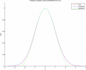
This comparison can be made more efficient with the "squeeze" $s(x)=(1-0.0331x^4)e^{-\frac{1}{2}x^{2}}\leq p(x)\leq e^{-\frac{1}{2}x^{2}}$, with an easily computable acceptance ratio, such that there is low probability of the squeeze being rejected when the true sample should be accepted. For $\alpha=2$ the acceptance ratio is about 98.1%. These distributions are shown graphically below.

An exponential family parametrized by $\boldsymbol\theta \in \mathbb R^d$ is the set of probability distributions that can be expressed as

\[ p({\bf x} \,|\, \boldsymbol\theta) =\frac{1}{Z(\boldsymbol\theta)} h({\bf x}) \exp\left( \boldsymbol\theta^{\mathsf T}\boldsymbol\phi({\bf x}) \right) ,\]

for given functions $Z(\boldsymbol\theta)$ (the partition function), $h({\bf x})$, and $\boldsymbol\phi({\bf x})$ (the vector of sufficient statistics). Exponential families can be discrete or continuous, and examples include Gaussian distributions, Poisson distributions, and gamma distributions. Exponential families have a number of desirable properties. For instance, they have conjugate priors and they can summarize arbitrary amounts of data using a fixed-size vector of sufficient statistics. But in addition to their convenience, their use is theoretically justified.

Suppose we would like to find a particular probability distribution $p({\bf x})$. All we know about $p({\bf x})$ is that $\mathbb E_{p({\bf x})}[f_k] = c_k$ for a specific collection of functions $f_1, \ldots, f_K$. Which distribution should we use? The principle of maximum entropy asserts that when choosing among all valid distributions, we should choose the one with maximum entropy. In other words, we should choose the distribution which has the greatest uncertainty consistent with the constraints.

For simplicity, consider the case in which $p({\bf x})$ is a distribution over a finite set $\{x_1, \ldots, x_J\}$. Then $p({\bf x})$ can be written as a vector $(p_1, \ldots, p_J)$. We would like to maximize

\[ -\sum_{j} p_j \log p_j \]

subject to the constraints $\sum_j p_j = 1$ and $\sum_j p_j f_k(x_j) = c_k$. Defining the quantity

What's learning theory good for, anyway? As I mentioned in my earlier blog post, not infrequently get into conversations with people in machine learning and related fields who don't see the benefit of learning theory (that is, theory of learning). While that post offered one specific piece of evidence of how work seemingly only relevant in pure theory could lead to practical algorithms, I thought I would talk in more general terms why I see learning theory as a worthwhile endeavor.

There are two main flavors of learning theory, statistical learning theory (StatLT) and computational learning (CompLT). StatLT originated with Vladimir Vapnik, while the canonical example of CompLT, PAC learning, was formulated by Leslie Valiant. StatLT, in line with its "statistical" descriptor, focuses on asymptotic questions (though generally based on useful non-asymptotic bounds). It is less concerned with computational efficiency, which is where CompLT comes in. Computer scientists are all about efficient algorithms (which for the purposes of theory essentially means polynomial vs. super-polynomial time). Generally, StatLT results apply to a wider variety of hypothesis classes, with few or no assumptions made about the concept class (a concept class refers to the class of functions to which the data generating mechanism belongs). CompLT results apply to very specific concept classes but have stronger performance guarantees, often using polynomial time algorithms. I'll do my best to defend both flavors, while also mentioning some of their limitations.

So, what is learning theory good for? I think there are both practical and philosophical reasons, four of which I will discuss below. At the end, I'll mention some of the major areas where existing theories fall short.

1. The occasional very practical algorithm. The regret/risk bounds and algorithms derived in the pursuit of  (or based on) theoretical guarantees can lead to practical algorithms. In the case of StatLT, there is Vapnik's structural risk minimization (SRM) framework, which provides generalization guarantees in terms of risk bounds. SRM led to the development of support vector machines, which have proven very useful in practice, independent of their theoretical properties. SVMs are a popular out-of-the-box classifier option since they require minimal tuning and, with the proper precautions, work quite well on most data sets. Hence, for many practitioners,  the cost of searching out the optimal classifier solution greatly outweighs the marginal improvement in performance that method would provide over SVMs. As for CompLT, the question of turning "weak learners" (learners that classify better than random chance) into "strong learners" (learners that can classify with arbitrarily small probability of error, given enough data) led to boosting methods, with AdaBoost (due to Freund and Schapire) being of particular note.  Other interpretations of AdaBoost have been developed which make it relevant even for algorithms that aren't "weak learners." For example, in an StatLT framework, boosting can also be viewed as finding the risk minimizer for a exponential loss from among a convex set of functions (a result due to Zhang [pdf]). I think an argument could be made the SVMs and AdaBoost alone justify the existence of learning theory. But I don't need defend such a bold statement, since I still have three more points discuss!

2. Formalizing what is "learnable." This argument is analogous to one of the arguments for studying complexity theory. Namely, that it's important to know which problems can't be solved efficiently. Think of all the wasted effort if researchers were spending valuable time trying to find a polynomial time algorithm for traveling salesman. Until the incredibly unlikely that a theorist comes along and proves P = NP, the world is quite content to find approximation algorithms or solve special cases. Analogously, results on the hardness of learning tell us which classes of functions are (likely to be) difficult to learn. For example, $\text{poly}(n)$-sized boolean formulas can't be PAC-learned in $\text{poly}(n)$ time. Such a result esnures we should either (a) give up on learning $\text{poly}(n)$-sized boolean formulas or (b) consider an alternative framework with a looser definition of what it means to learn. Thus, these results help guide our thinking about what can be realistically learned and what we even mean by learning.

3. Intuition about what learning rates we can hope to achieve. This argument has a similar flavor to #2, but I separate it out because whereas #2 is about theorems and specific results, this is about gaining conceptual insight that is independent of a particular problem. For example, in both StatLT and CompLT, results are usually phrased as holding "with high probability" (i.e. with probability greater than $1-\delta$). Both theories show that the sample complexity "should" scale like $\text{poly}(\log(1/\delta))$. There's a very simple, general argument for why this should be, but nonetheless it's worth keeping in mind because it tells us that our main concern shouldn't be what happens if we get unlucky (with unrepresentative data). We can make the probability of that exponentially small at only a polynomial cost. Our real concern should be our "error" parameter, call it $\epsilon$, for which sample complexity scales like $\text{poly}(1/\epsilon)$. There's good reason to think this should hold –– we can't expect the amount we learn to increase exponentially with the amount of data. Specific theories and situations can provide more fine-grained intuition. For example, StatLT tells us risk/error bounds usually decrease like $1/\sqrt{n}$. Such understanding can provide realistic expectations of what might happen if, say, we double the amount of labeled data we have (in this case, we should expect only a $1/\sqrt{2}$ factor decrease in ``$\epsilon$'', not a $1/2$).

4. Controlling model complexity and Occam's razor-like results. Many theorems in CompLT and StatLT provide instantiations of Occam's razor: “The simpler explanation is to be preferred."* The simplest version of this, from PAC learning, is known as "Occam's razor theorem." Roughly speaking, it states we don't want to choose from too many hypotheses compared to the amount of data we have. In particular, we want the size of the hypothesis space used to grow like $2^{\Theta(m)}$, where $m$ is the number of data points we are trying to explain. Note that there are $2^{2^n}$ possible boolean functions on $n$ binary variables, so exponential growth is actually slow. The myriad results in both CompLT and StatLT that rely on various measures of the complexity of hypothesis classes --- such as VC dimension, fat-shattering dimension, Rademacher and Gaussian complexity, and covering numbers --- generalize the simple PAC Occam's razor result to realistic scenarios in which the hypothesis class has uncountably many functions. These complexity measures have many close connections with each other. Combined the risk bounds and lower bounds on learning rates they appear in, they can help us to understand and compare different hypothesis classes for which size and number of parameters are not good measures of complexity. A canonical example of the number of parameters being a bad measure of complexity is that the sine function (1 parameter) has infinite VC dimension while a $d$-dimensional hyperplane ($d$ parameters) has VC dimension $d$. A practical example where complexity measures  provide important insight come from kernel learning methods, which project data into an infinite-dimensional space. The fact that such methods work would seem to suggest they are magically avoiding the "curse of dimensionality." But by looking at complexity measures for specific kernels, one finds that their effective dimensionality is very much finite. As a representative example, Zhang (2005) [pdf] shows that the effective dimension for kernel regression with an exponential kernel is $O(\ln n / \ln \ln n)$, where $n$ is the number of data points.

So there you go. I hope I've convinced the unbelievers and skeptics that learning theory does in fact offer significant value to those interested in practical learning question. Clearly, it is not a panacea and fails to capture important aspects of real-world learning problems. There are many algorithms that work well in practice for which we have no theoretical justification. But, as far as I'm concerned, such shortcomings are good justification for continuing to work on developing better theory.

*In the interest of completeness, I should mention that outside CompLT and StatLT, there's also the "Bayesian Occam's razor" theorem that gets at the same idea for Bayesian inference.

The purpose of this post is to present the very basics of potential theory for finite Markov chains. This post is by no means a complete presentation but rather aims to show that there are intuitive finite analogs of the potential kernels that arise when studying Markov chains on general state spaces. By presenting a piece of potential theory for Markov chains without the complications of measure theory I hope the reader will be able to appreciate the big picture of the general theory.

This post is inspired by a recent attempt by the HIPS group to read the book "General irreducible Markov chains and non-negative operators" by Nummelin.

Let $P$ be the transition matrix of a discrete-time Markov chain on a finite state space such that $p_{ij}$ is the probability of transitioning from state $i$ to state $j$. We call a Markov chain absorbing if there is at least one state such that the chain can never leave that state once entered. Such a state is called an absorbing state, and non-absorbing states are called transient states. An ergodic Markov chain is such that every state is reachable from every other state in one or more moves. A chain is called a regular Markov chain if all entries of $P^n$ are greater than zero for some $n$. We will focus on absorbing chains first, and then look at ergodic and regular chains.

By permuting the states of an absorbing chain so that the transient states come first, we can write the transition matrix of the absorbing chain as
\begin{equation}
P = \left [ \begin{array}{cc}
Q & R \\
0 & I
\end{array} \right ]
\end{equation}
The matrix $Q$ describes the transition probabilities between transient states, $R$ the transition probabilities from transient to absorbing states ($R$ should not be the matrix of all zeros), and $I$ is the identity matrix since the chain stays at absorbing states.

Notice that the iterates $Q^n \rightarrow 0$ as $n \rightarrow \infty$. We can see this by noting that the probability that the chain does not reach an absorbing state from a transient state is the sum of the corresponding row of $Q$, call it $q_j$. The probability of not being absorbed in $n$ steps is $q_j^n$, and since $q_j < 1$ this probability goes to $0$ so the individual entries of $Q^n$ converge to $0$ as well. We define the fundamental matrix for an absorbing Markov chain as
\begin{equation}
N = I + Q + Q^2 + \ldots
\end{equation}
Each entry of $N$, $n_{ij}$, can be interpreted as the expected number of times the chain is in state $j$ if it started in state $i$. Note that $N$ is the finite analog of the potential kernel $G$ from Nummelin, and it can be shown that $N = (I-Q)^{-1}$.

The fundamental matrix, $N$, can be used to compute many interesting quantities of an absorbing Markov chain (which probably explains the name fundamental matrix). For instance, we can compute the expected time until the chain is absorbed as $t = N1$, where $t = (t_1,\ldots,t_K)$ is a vector where $t_i$ is the expected number of steps until the chain reaches an absorbing state starting from state $i$, and $1$ is a vector of ones. We can also compute the probability that a particular absorbing state is reached given a starting state. Let $B$ be a matrix where $b_{ij}$ is the probability of reaching absorbing state $j$ starting at state $i$. It turns out that $B=NR$, where $R$ is in the decomposition of $P$ above.

Now we turn our attention to ergodic and regular Markov chains. Let $P$ be the transition matrix of a regular Markov chain, then the iterates, $P^n$ converge to a matrix, $W$, such that all rows of $W$ are the same. Call the shared row $w$ so that $w = Pw$. The vector $w$ is called the stationary distribution of the chain. We can also define a fundamental matrix for ergodic and regular Markov chains.

As a first attempt at the form of the fundamental matrix for an ergodic or regular chain we could try $N = (I - P)^{-1}$. However, $(I-P)$ does note have an inverse since the columns are linearly dependent. The reason we could define $N$ for absorbing chains was because the iterates $Q^n$ were decaying to $0$. Since $P^n \rightarrow W$, we may instead try defining
\begin{equation}
N = I + (P-W) + (P-W)^2 + \ldots
\end{equation}
The terms in this series decay to $0$ and the series ends up converging. We then have $N = (I-P+W)^{-1}$ is the fundamental matrix of an ergodic or regular chain.

As in the absorbing case $N$ can be used to compute some interesting properties of the chain. For instance, the mean first passage time is the expected number of steps required to reach state $j$ from state $i$ which we denote by $m_{ij}$. It can be shown that $m_{ij} = \frac{n_{jj} - n_{ij}}{w_j}$. The fundamental matrix also appears in the asymptotic variance in the Central Limit Theorem for Markov chains.

I highly recommend reading Chapter 11 from "Introduction to Probability" by Grinstead and Snell (available for free here) for a nice introduction to finite Markov chains. It is written at the undergraduate level, but it is very clear and contains some ideas and results that you probably didn't see in your first treatment of Markov chains. Another nice reference for finite Markov chains that covers potential theory is "Finite Markov Chains" by Kemeny and Snell.

As a quick aside, notice that the fundamental matrices defined here are the inverses of matrices that look very similar to graph laplacians. The short story is that potential theory for Markov chains (and processes more generally) is related to classical potential theory in physics. In fact there is a deep connection between Markov chains and electric networks. See this book by Doyle and Snell for a treatment.

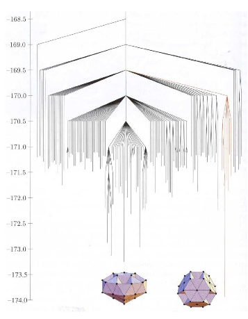
I would like to briefly introduce disconnectivity graphs -- striking visualizations of multidimensional energy landscapes that I had never seen before. While it's not immediately obvious how useful they are, it should be straightforward to adapt them for visualizing probability distributions.

A quick Google search for 'disconnectivity graph' will turn up lots of examples. These things look like chandeliers and are meant to summarize the potential energy surface of a molecule, potentially with many degrees of freedom and many local optima -- think of trying to describe the energies of all of the configurations of a floppy protein or nanodroplet of water. Physicists like David Wales, who gave a talk yesterday on "Exploring Energy Landscapes", use disconnectivity graphs to gain intuition about how (local) minima are connected within such a system and how fast a system will reach the global minimum. You should soon be able to access his talk through the IACS video archive.

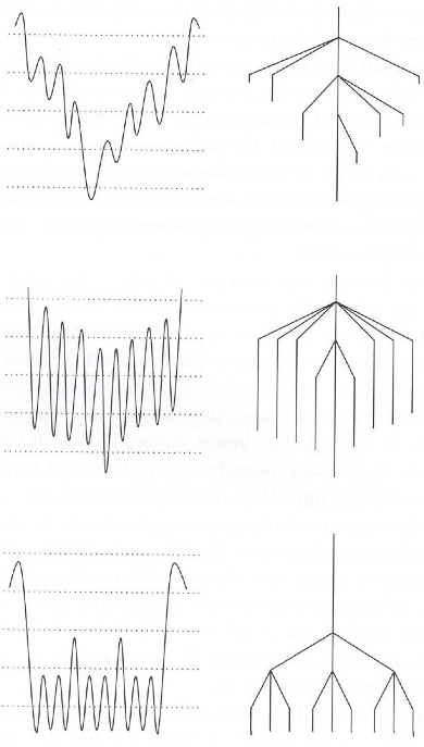
I'll briefly describe how to construct a disconnectivity graph, which should make their interpretation clear. Alternatively, check out this nice summary. The idea is to analyze the landscape with respect to a sequence of energies. Think of a particular energy E as a (hyper)plane slicing through the landscape at a constant height and now flood the landscape from below with water up to this level. Some of the minima are above the water and the rest are partitioned according to separate pools of water. The minima within each pool form 'superbasins' -- sets of minima that are connected by pathways whose energies are below E. A disconnectivity graph is a tree that shows the number of superbasins present at a discrete set of energies (heights) and its branching structure as you move down the graph shows how superbasins at one energy are related to those at the next lower energy. At high enough energies, all the minima are contained in one superbasin (the top of the tree) and the ends of the branches correspond to the energies of the minima. The horizontal spacing of the branching is arbitrary.

For visualizing probability distributions, we basically want to flip the energy analogy upside down since we tend to care about the maxima rather than the minima. An obvious caveat with all of this is that in general, we don't know where all of the optima are! My understanding of what the physicsts do is to use local minimization routines to search for minima and then hope for the best.

Figures from: David J. Wales. Energy landscapes: With applications to clusters, biomolecules and glasses. Cambridge University Press, ISBN 0-521-814157-4, 2003.