This is the second of two posts based on a testing tutorial I'm writing with David Duvenaud.

In my last post, I talked about checking the MCMC updates using unit tests. Most of the mistakes I've caught in my own code were ones I caught with unit tests. (Naturally, I have no idea about the ones I haven’t caught.) But no matter how thoroughly we unit test, there are still subtle bugs that slip through the cracks. Integration testing is a more global approach, and tests the overall behavior of the software, which depends on the interaction of multiple components.

When testing samplers, we’re interested in testing two things: whether our algorithm is mathematically correct, and whether it is converging to a correct solution. These two goals are somewhat independent of each other: a mathematically correct algorithm can get stuck and fail to find a good solution, and (counterintuitively) a mathematically incorrect algorithm can often find the correct solution or at least get close. This post is about checking mathematical correctness.

The gold standard for testing MCMC algorithms is the Geweke test, as described in Geweke’s paper “Getting it right: joint distribution tests of posterior simulators.” [1] The basic idea is simple: suppose you have a generative model over parameters $\theta$ and data $x$, and you want to test an MCMC sampler for the posterior $p(\theta | x)$. There are two different ways to sample from the joint distribution over $\theta$ and $x$. First, you can forward sample, i.e. sample $\theta$ from $p(\theta)$, and then sample $x$ from $p(x | \theta)$. Second, you can start from a forward sample, and run a Markov chain where you alternate between

1. Updating $\theta$ using one of your MCMC transition operators, which should preserve the distribution $p(\theta | x) $, and
2. resampling the data from the distribution $p(x | \theta) $.

Since each of these operations preserves the stationary distribution, each step of this chain is a perfect sample from the joint distribution $p(\theta, x)$.

If your sampler is correct, then each of these two procedures should yield samples from exactly the same distribution. You can test this by comparing a variety of statistics of the samples, e.g. the mean of $x$, the maximum absolute value of $\theta$, and so on. No matter what statistics you choose, they should be indistinguishable between the two distributions.

The beauty of this approach is that it amplifies subtle bugs in the sampler. For instance, suppose we have a bug in our sampler which makes the posterior noise variance 1% too large. This would be nearly impossible to detect by simply running your model on real data and seeing if the results look plausible. Now consider what the Geweke test would do. After the parameters are sampled, the data will be generated with a 1% larger noise variance. When the parameters are resampled, the noise variance will be 1% too large on top of that, or 2%. Pretty soon, the noise variance will explode.

In his paper, Geweke uses frequentist hypothesis tests to compare the distributions. This can be difficult, however, since you’d need to account for dependencies between the samples in order to determine significance. A simpler approach is to make a P-P plot of the statistics. If it’s very close to a straight line, the test "passes":

 If it’s far off, you have a bug:

If the results are noisy and unclear, generate more forward samples and run the chains for longer:

(While these figures are synthetic, they're representative of outputs I've gotten in the past.) If you wind up with the third case, and you can't run the sampler any longer because it's already too slow, try reducing the number of data points. Not only does this speed up each iteration, but it also makes the chains mix faster -- the more data points there are, the stronger the coupling between $\theta$ and $x$.

There’s a major drawback of the Geweke test, unfortunately: it gives you no indication of where the bug might be. All you can do is keep staring at your code till you find the bug. Therefore, there’s no point in running this test until all your unit tests already pass. This meshes with the general test-driven development methodology, where you get your unit tests to pass before the integration tests.

[1] J. Geweke. Getting it right: joint distribution tests of posterior simulators. JASA, 2004.

Here's an interesting question: how much space would it take to store the genomes of everyone in the world? Well, there are about 3 billion base pairs in a genome, and at 2 bits per base (4 choices), we have 6 billion bits or about 750 MB (say we are only storing one copy of each chromosome). Multiply this by 7 billion people and we have about 4800 petabytes. Ouch! But we can do a lot better. We know that genomes of different humans are very similar; let's say 99.9% similar. For the calculations that follow I'll make the simplifying assumption that there exists some prototype genome, and that all other human genomes differ from it by exactly 0.1%, that is to say they differ from it at exactly 3 million locations. I will also assume that all allowed genomes are equally likely.

How do we use this assumption to compress genomes? First, consider the following simple scheme: we store the prototype genome, and then for each new genome, we store the locations of the changes, and the changes themselves. Since $2^{32}$ is about 4 billion, a regular 32 bit integer is enough to store the change locations. Then let's use an extra 2 bits to store the actual new base, for a total of 34 bits per change. With 3 million changes, this gives us a size of about 3 million $\times$ 34 bits = 13 MB per genome. That's already a lot better than 750 MB. But, can we do better? (Notation pit-stop: I will use the shorthand M for million and B for billion... but MB is still megabyte! I will use $\lg$ to mean log base 2.)

Luckily, Shannon figured out the theoretical limit on how much we can compress things. According to Shannon, since every allowed genome is assumed to be equally likely, all we need to do is count the number of allowed genomes and then take the log. The number of possible sets of change locations is $\binom{3B}{3M}$, or "3 Billion choose 3 Million", because we need to pick 3M change locations of out 3B possible locations. For each of these sets, we need to choose the new bases themselves, and there are 3 choices per base. So the total number of possible allowed genomes is \[\binom{3B}{3M} 3^{3M} = \frac{3B!}{3M! (3B-3M)!} 3^{3M}= \frac{3B!}{3M! 2.997B!} 3^{3M}\] Now, we take the log of this to get the minimum file size: \[\lg{3B!}-\lg{3M!}-\lg{2.997B!}+3M\lg{3}\]Using Stirling's formula, $\log{n!}\approx n\log{n}$, this gives us \[3B\lg{3B}-3M\lg{3M}-2.997B\lg{2.997B}+3M\lg{3}\](Note: I only kept the first term in Stirling's approximation. It turns out that the next term cancels out in this case, so I skipped it for the sake of cleanliness.) From here we can just compute the result with a normal calculator and we get about 39 million bits, or about 5 MB.

What does this mean? When we took advantage of the similarity of genomes, we compressed from 750 MB to 13 MB (about 90 PB for 7 billion people, down from 4800 PB). But the calculation above says that the theoretical limit is 5 MB. Why is our algorithm 8 MB shy of the optimum? In other words, from an intuitive point of view, where is the "slack" in our method? You might enjoy thinking about this for a minute before reading on.

I have identified 3 sources of slack in the above algorithm.

1. We used 2 bits for every base change, but actually there are only 3 possibilities for a change, not 4. So, theoretically, we only need $\lg{3}\approx 1.6$ bits per change, instead of 2 bits.
2. (a) We used 32 bits to store each change location (which is a number between 1 and 3 billion), but actually we only need $\lg(3B)\approx 31.5$ bits. (b) Furthermore, we don't even need this many $(\lg 3B)$ bits every time: the first time we need a number between 1 and 3B, but next time we only need to choose between 3B-1 locations, and then 3B-2, etc. since there are no repeats.
3. The set of changes is sent in a particular order, which is irrelevant. We could permute the list of changes, and the resulting genome would be the same.

The next question is: what is the size of each of these effects? I will address these in the same order as they appear above.

1. Using 2 bits instead of $\lg{3}$ bits per change has a total waste per genome of $3M\cdot (2-\lg{3})$ which is about 1.2 million bits or 0.15 MB.
2. (a) Using 32 bits instead of $\lg{3B}\approx 31.5$ bits per change has a total waste per genome of $3M (32-\lg{3B})$, which is about 1.6 million bits or 0.19 MB.
   (b) The size of effect 2(b) is the difference between sending $\lg{3B}$ bits 3 million times and the slightly more optimal version of sending $\lg{3B}$ bits, then $\lg{(3B-1)}$, and so on until $\lg{2.997B}$ bits for the last change location. Mathematically, this difference is \[(3M\cdot\lg{3B})-(\lg{3B}+\lg{(3B-1)}+ \ldots + \lg{2.997B})\]This effect is very tiny, only about 2000 bits or 0.00025 MB.
3. Sending an ordered list when ordering is not necessary means that all possible orderings of the 3M changes produce the same result. Since there are $3M!$ possible orderings of 3M changes, there is a redundancy factor of $3M!$ in this method. Thus the ordering has a waste of $\lg{3M!}$ bits. Here I again need Stirling's formula, and this time I will keep the second term because it does not cancel. Stirling's formula says\[\log{n!}\approx n\log{n}-n=n\log{(n/e)}\]We can again change this to log base 2 because the correction factor cancels from both sides, so we have\[\lg{3M!}\approx 3M\lg{(3M/e)}\]which is about 60 million bits or 7.5 MB.

Let's take a moment to interpret these results. First, it's interesting that almost all of the slack comes from the ordering issue, slack source #3. This was not very intuitive to me at first; it seems like such an abstract concept that "we send things in some particular order but actually the order doesn't matter", but this "abstract" concept costs us 7.5 MB, or about 52 petabytes for all 7 billion genomes. Hopefully this issue will become more clear in the following paragraphs.

Second, did we find all of the slack? The original algorithm was 13 MB (actually 12.75 MB) and the theoretical limit was 5 MB (actually 4.87 MB). We found a total of 0.15 MB + 0.19 MB + 0.00025 MB + 7.53 MB = 7.87 MB of slack. Add this to the theoretical limit of 4.87 MB and we get 12.74 MB. This seems plausibly within rounding error of 12.75 MB, which is great! But, maybe we still missed something?

The answer is that we did not miss anything. Below, I will show definitively that we found all the slack. In particular, I will show how, starting with the mathematical expression for the theoretical minimum, $\lg{3B!}-\lg{3M!}-\lg{2.997B!}+3M\lg{3}$ bits, we can act on it with each slack source in turn and end up with the exact mathematical expression for our algorithm, $3M\cdot32 + 3M\cdot2$ bits. Here we go... [it is possible to skip the next 3 paragraphs if you believe me and do not need to see the calculations]

First, we apply slack source 1, which connects the $3M\lg{3}$ term to the $3M\cdot 2$ term. Slack source 1 says that there are only 3 choices for a change of base, not 4. This corresponds exactly to changing the $\lg{3}$ to $\lg{4}=2$ for each change, or $3M\lg{3}$ to $3M\lg{4}=3M\cdot 2$ bits in total.

Next we apply slack source 2, which connects $\lg\frac{3B!}{2.997B!}$ to $3M\cdot 32$. We start with slack source 2(b). In the theoretical calculation we started with the ratio $\frac{3B!}{2.997B!}$, which is the same as $3B\times (3B-1)\times ... \times 2.997B$. This product is fairly similar to $3B\times 3B\times ... \times 3B$, or $(3B)^{3M}$. Indeed, the mathematical approximation $\frac{3B!}{2.997B!}\approx3B^{3M}$ exactly corresponds to slack 2(b): it is the intuitive approximation that it is OK to just send $\lg{3B}$ bits per change location, instead of the slightly optimized version described above. Then, from there, $\lg{(3B)^{3M}}=3M\lg{3B}$, and effect 2(a) above says that we approximate $\lg{3B}$ as 32. When we apply this approximation, we get $3M\cdot 32$, which is exactly the term we were looking for.

Finally, we apply slack source 3. The only term left in the theoretical formula is the $3M!$ in the denominator, which has no corresponding term in the formula for our algorithm. This is exactly slack source 3, as described earlier! The slack due to ordering has a redundancy of $3M!$ possible orderings, and when we divide this out in the "choose" formula, this exactly corresponds to saying that, in theory, we do not need ordering, so we divide these permutations out, thus reducing the theoretical limit by exactly $\lg{(3M!)}$ bits.

To recap: I have now shown that the formula for the size of our algorithm can be obtained by starting with the theoretical formula and applying a series of mathematical approximations, and furthermore that each of these approximations exactly corresponds to one of the intuitive slack sources described above. Thus, we have "found" all the slack; i.e. we have an intuitive understanding of all the reasons why our method for storing genomes compresses less than the theoretical limit.

I want to add one last chapter to the story, namely to address the obvious question: "What is a better algorithm that performs closer to the theoretical limit?" One intuitive answer is the following: instead of encoding the change locations explicitly, encode the distances ("diffs") between subsequent change locations. For example, instead of transmitting that there are changes at locations 195, 200, and 240, just encode "195", "5", and "40". Intuitively, these diffs will be small, on average 1000 or so. By transmitting smaller numbers, we can save bits. Using our newfound intuition, we can also say definitively that encoding the diffs eliminates the order-based slack, because the diffs must be sent in the proper order for the answer to be correct. [Note: the discussion below about diffs is meant to illustrate the intuitions described above, and is not necessarily the best solution. To solve this problem more optimally, I would probably use arithmetic coding. A new method for compressing unordered sequences is described in this paper.]

To make this more concrete, I propose the following algorithm: sort the locations of all the changes and find the diffs. Then, use $n<32$ bits to encode each diff. If a particular diff requires more than $n$ bits (i.e., is $\geq 2^n$), then we will send a special symbol of $n$ zeros, followed by the full 32-bit representation of the diff. How do we choose $n$? Intuitively, if we pick $n$ too small then almost all of the diffs will overflow and we will end up sending them as full 32-bit representations, gaining nothing. On the other hand, if $n$ is too large then we don't get significant gains because the diffs are sent with more bits than needed. Thus we can expect some middle ground that gives the best performance.

To test this, I implemented a codec using this method. I first generated random genomes using the assumptions above, then compressed them with this method and plotted the performance as a function of $n$. The results are shown in the figure below. (Code is posted here.)

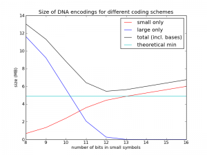
The cyan line is the theoretical limit, at about 4.9 MB. The red line shows just the size of the diffs represented with $n$ bits. The blue line shows just the size of the diffs represented with $n+32$ bits (the "overflows"). The black line is the sum of the red line, the blue line, and the $3M\cdot 2$ bits used for the new bases (as you can see, I didn't bother addressing slack source 1, but at least now I know it only costs me 0.15 MB per genome). What we see is just what we expected: things get worse, and then they get better. In this case we see the best value is $n=12$, and its size is about 5.4 MB, quite close to the theoretical limit.

To improve a diff-based system further, one would have to take into account the probability distribution of the diffs. Below is an empirical histogram of this distribution from one random genome I generated. (Quick sanity check: the picture is approximately a triangle with base length 2000 and height 0.001, so its area is plausibly equal to 1). Intuitively, the algorithm above is optimal for a distribution that is different from this one. In particular, the algorithm "thinks" the distribution is a piece-wise constant function with two pieces, one higher-probability piece between 1 and $2^n-1$ and another, lower-probability piece from $2^n$ to 3B. Changing $n$ changes the shapes of these steps, and presumably choosing $n=12$ maximizes the "overlap" between the implied piece-wise distribution and the real distribution (approximately) shown here.

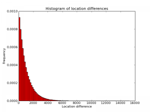
Comments, questions, or corrections? Please email me! My email is listed near the top of my website.

This post is taken from a tutorial I am writing with David Duvenaud.

Overview

When you write a nontrivial piece of software, how often do you get it completely correct on the first try?  When you implement a machine learning algorithm, how thorough are your tests?  If your answers are "rarely" and "not very," stop and think about the implications.

There's a large literature on testing the convergence of optimization algorithms and MCMC samplers, but I want to talk about a more basic problem here: how to test if your code correctly implements the mathematical specification of an algorithm. There are a lot of general strategies software developers use to test code, but machine learning algorithms, and especially sampling algorithms, present their own difficulties:

• The algorithms are stochastic, so there's no single "correct" output
• Algorithms can fail because they get stuck in local optima, even if they are mathematically correct
• Good performance is often a matter of judgment: if your algorithm gets 83.5% of the test examples correct, does that mean it's working?

Furthermore, many machine learning algorithms have a curious property: they are robust against bugs. Since they’re designed to deal with noisy data, they can often deal pretty well with noise caused by math mistakes as well. If you make a math mistake in your implementation, the algorithm might still make sensible-looking predictions. This is bad news, not good news. It means bugs are subtle and hard to detect. Your algorithm might work well in some situations, such as small toy datasets you use for validation, and completely fail in other situations -- high dimensions, large numbers of training examples, noisy observations, etc. Even if it only hurts performance by a few percent, that difference may be important.

If you're a researcher, there's another reason to worry about this. Your job isn’t just to write an algorithm that makes good predictions -- it’s to run experiments to figure out how one thing changes as a result of varying another. Even if the algorithm “works,” it may have funny behaviors as some parameterizations compensate for mistakes better than others. You may get curious results, such as performance worsening as you add more training data. Even worse, you may get plausible but incorrect results. Even if these aren’t the experiments you eventually publish, they’ll still mess up your intuition about the problem.

In the next two blog posts, I'll focus on testing MCMC samplers, partly because they're the kind of algorithm I have the most experience with, and partly because they are especially good illustrations of the challenges involved in testing machine learning code. These strategies should be more widely applicable, though.

In software development, it is useful to distinguish two different kinds of tests: unit tests and integration tests. Unit tests are short and simple tests which check the correctness of small pieces of code, such as individual functions. The idea is for the tests to be as local as possible -- ideally, a single bug should cause a single test to fail. Integration tests test the overall behavior of the system, without reference to the underlying implementation. They are more global than unit tests: they test whether different parts of the system interact correctly to produce the desired behavior. Both kinds of tests are relevant to MCMC samplers.

A development pattern called test-driven development is built around testability: the idea is to first write unit and integration tests as a sort of formal specification for the software, and then to write code to make the tests pass. A fully test-driven development process might look something like:

1. write integration tests based on high-level specs for the system
2. write unit tests
3. write code which makes the unit tests pass
4. make sure the integration tests pass

In research, because the requirements are so amorphous, it is often difficult to come up with good specs in advance. However, I've found the general idea of getting unit tests to pass, followed by integration tests, to be a useful one. I'll talk about unit tests in this blog post and integration tests in the followup.

Unit testing

Unit testing is about independently testing small chunks of code. Naturally, if you want to unit test your code, it needs to be divided into independently testable chunks, i.e. it needs to be modular. Such a modular design doesn’t happen automatically, especially in research, where you’re building up a code base organically with constantly shifting goals and strategies. It can be difficult to retrofit to code base with unit tests; in fact, the book Working effectively with legacy code defines legacy code as “code without unit tests.” The whole book is about strategies for refactoring an existing code base to make it testable.

It’s much easier to try to keep things modular and testable from the beginning. In fact, one of the arguments behind test-driven development is that by writing unit tests along with the actual code, you force yourself to structure your code in a modular way, and this winds up having other benefits like reusability and maintainability. This agrees with my own experience.

Unfortunately, the way machine learning is typically taught encourages a programming style which is neither modular nor testable. In problem sets, you typically work through a bunch of math to derive the update rules for an iterative algorithm, and then implement the updates directly in MATLAB. This approach makes it easy for graders to spot differences from the correct solution, and you’ll probably be able to write a correct-looking homework assignment this way, but it’s not a robust way to build real software projects. Iterative algorithms are by nature difficult to test as black boxes.

Fortunately, most machine learning algorithms are formulated in terms of general mathematical principles that suggest a modular organization into testable chunks. For instance, we often formulate algorithms as optimization problems which can be solved using general techniques such as gradient descent or L-BFGS. From an implementation standpoint, this requires writing functions to (a) evaluate the objective function at a point, and (b) compute the gradient of the objective function with respect to the model parameters. These functions are then fed to library optimization routines. The gradients can be checked using finite difference techniques. Conveniently, most scientific computing environments provide implementations of these checks; for instance, scipy.optimize.check_grad (in Python) or Carl Rasmussen’s checkgrad function (in MATLAB).

This organization into gradient computations and general purpose optimization routines exemplifies a generally useful pattern for machine learning code: separate out the implementations of the model and general-purpose algorithms. Consider, for instance, writing a Gibbs sampler for a distribution. Seemingly the most straightforward way to implement a Gibbs sampler would be to derive by hand the update rules for the individual variables and then write a single iterative routine using those rules. As I mentioned before, such an approach can be difficult to test.

Now consider how we might separate out the model from the algorithm. In each update, we sample a variable $X$ from its conditional distribution $p(X|Z)$. It is difficult to directly test the correctness of samples from the conditional distribution: such a test would have to be slow and nondeterministic, both highly undesirable properties for a unit test to have. A simpler approach is to test that the conditional distribution is consistent with the joint distribution. In particular, for any two values $X$ and $X^\prime$, we must have:

$\frac{p(X^\prime | Z)}{p(X | Z)} = \frac{p(X^\prime, Z)}{p(X, Z)}$

Importantly, this relationship must hold exactly for any two values $X$ and $X^\prime$. For the vast majority of models we use, if our formula for the conditional probability is wrong, then this relationship would almost surely fail to hold for two randomly chosen values. Therefore, a simple and highly effective test for conditional probability computations is to choose random values for $X$, $X^\prime$, and $Z$, and verify the above equality to a suitable precision, such as $10^{-10}$. (As usual in probabilistic inference, we should use log probabilities rather than probabilities for numerical reasons.)

In terms of implementation, this suggests writing three separate modules:

1. classes representing probability distributions which know how to (1) evaluate the log probability density function (or probability mass function) at a point, and (2) generate samples
2. a specification of the model in terms of functions which compute the probability of a joint assignment and functions which return conditional probability distributions
3. a Gibbs sampling routine, which sweeps over the variables in the model, replacing each with a sample from its conditional distribution

The distribution classes require their own forms of unit testing. For instance, we may generate large numbers of samples from the distributions, and then ensure that the empirical moments are consistent with the exact moments. I'll defer discussion of testing the Gibbs sampler itself to my next post.

While this modular organization was originally motivated by testability, it also has benefits in terms of reusability: it’s easy to reuse the distribution classes between entirely different projects, and the conditional probability functions can be reused in samplers which are more sophisticated than Gibbs sampling.

While Gibbs sampling is a relatively simple example, this thought process is a good way of coming up with modular and testable ways to implement machine learning algorithms. With more work, it can be extended to trickier samplers like Metropolis-Hastings. The general idea is to make a list of mathematical properties that the component functions should satisfy, and then check that they actually satisfy those properties.

There are a lot of helpful software tools for managing unit tests. I use nose, which is a simple and elegant testing framework for Python. In order to avoid clutter, I keep the tests in a separate directory whose structure parallels the main code directory.

I've found that unit testing of the sort that I've described takes very little time and provides substantial peace of mind. It still doesn't guarantee correctness of the full algorithm, of course, so in the next post I'll talk about integration testing.

The proof and intuition presented here come from this excellent writeup by Yuval Filmus, which in turn draws upon ideas in this book by Fumio Hiai and Denes Petz. Suppose that we have a sequence of real-valued random variables $X_1, X_2, \ldots$. Define the random variable

A few years ago MATLAB introduced a Just-In-Time (JIT) accelerator under the hood. Because the JIT acceleration runs behind the scenes, it is easy to miss (in fact, MathWorks seems to intentionally hide it so that users do not change their coding style, probably because the JIT accelerator is changed regularly). I just wanted to briefly mention what a JIT accelerator is and what it does in MATLAB. JIT compilers compile chunks of code at runtime, so instead of interpreting the MATLAB code line-by-line (the default for an interpreted language), it compiles certain chunks of code and then runs the compiled chunks as a block. The JIT acceleration in Matlab works quite well. I wrote the following code to demonstrate MATLAB's JIT in action:

N = 1e7;

I've recently come across a fascinating blog post by Cambridge mathematician Tim Gowers. He and computational linguist Mohan Ganesalingam built a sort of automated mathematician which does the kind of "routine" mathematical proofs that mathematicians can do without backtracking. Their system was based on a formal theory of the semantics of mathematical language, together with introspection into how they solved problems. In other words, they worked through lots of simple examples and checked that their AI could solve the problems in a way that was cognitively plausible. The goal wasn't to build a useful system (standard theorem provers are way more powerful), but to provide insight into our problem solving process. This post reminded me that, while our field has long moved away from this style of research, I think there's still a lot to be gained from it.

Introspection has a long and distinguished history in the early days of AI:

• Newell and Simon's General Problem Solver [1] was explicitly based on intuitions about how we solve problems, and they developed it by working through lots of examples by hand
• Lenat's Automated Mathematician [2] was supposed to make mathematical conjectures based on heuristics that human mathematicians followed
• Hofstadter's book Fluid Concepts and Creative Analogies [3] details AI systems which serve as cognitive models for a variety of toy problems. Some nice examples are Seek-Whence (for explaining number sequences) and Copycat (for letter string analogies).

Like Gowers's work, these classic systems were intended primarily as cognitive models. Simon was inspired to work on AI when he did consulting work on group decision making for the air force and found that he didn't have an adequate formalism for explaining their decision making process [4]. Lenat was at least partially motivated by formalizing Polya's notion of a heuristic, since he thought informal lists of heuristics probably oversimplified the process of mathematical discovery and suffered from hindsight bias [5]. The idea was that translating our own heuristics into mathematically precise algorithms gives a more rigorous way of testing which strategies are capable of solving which problems.

But introspection has largely fallen out of favor in AI, at least the parts I'm familiar with (machine learning, vision, probabilistic inference). The field has a Behaviorist-like aversion to thinking about algorithms in terms of plausible mental representations and cognitive strategies. I can think of several plausible arguments against introspection:

• We already have rough outlines of a solution for most of the problems we're interested in, and introspection won't help us fill in any of the details.
• Computers are a different enough computational architecture from the brain that we can't expect any insights to carry over. I.e., computers can perform billions of sequential operations per second (which often makes brute force a more viable strategy), whereas the brain has more effective associative memory and high-level representations.
• Introspection isn't scientific, since different people will disagree. The explanations are likely just someone's idealized story about what's actually a much messier process. (E.g., cognitive scientist Jeff Shrager spent three years training to be a molecular biologist, and during this time, he couldn't find any examples of the cross-domain analogies that cognitive scientists had touted as so fundamental to scientific discovery.)
• It's hard to predict what range of problems an introspection-based strategy will generalize to.

As far as the first point, I think there are still plenty of hard problems for which we don't even have the outlines of a solution. The remaining points seem hard to argue with, but they basically just show that introspection is a source of intuition rather than a rigorous way of evaluating algorithms. I'd say we have three major sources of intuition in our field:

1. trying out models and algorithms in a variety of settings, both real-world applications and toy problems
2. peer-reviewed research in cognitive science and neuroscience
3. introspection

Neuroscience and cog sci both had a large influence on both machine learning and computer vision in the early days, but as the field as matured, algorithms have made up a larger and larger part of our intuitions. Introspection is rarely mentioned.

In my own work on structure learning, my co-authors and I made several design decisions based on how human researchers would approach a problem. In my matrix decompositions work [6]:

• we often come up with structured probabilistic models by first fitting a simpler one to the data, seeing if there are dependencies in the learned representation which aren't captured by the model, and adding those explicitly to the model
• if we're trying to do inference in a complex probabilistic model, it often works to initialize it from a simpler one

And for Gaussian process structure search [7]:

• a good strategy for building up structured GP models is to try to model the residuals of the current model, and add the resulting kernel to the model
• when we use the above strategy, the previously learned kernel hyperparameters make a good initialization for the larger model

Of course, for the aspects of our algorithms that have already been well-explored (such as inference in particular models), we went with the standard approaches. There's no point in thinking, "How would I try to factorize this matrix..." But since hardly anyone has explored how to structure model spaces in a way that's searchable, these intuitions provided useful guidance in the design of our spaces of models.

Like any source of intuition, introspection is just a starting point. It's not a rigorous scientific argument, and it ultimately needs to be backed up with math and experiments. What we really want is an explanation for the heuristics people use. In other words,

1. figure out what regularities our heuristics are exploiting
2. see if existing algorithms already exploit those same regularities
3. if not, come up with one that does
4. justify it theoretically and empirically

You can think of this as a sort of "inverse Bayesian optimization." I'm currently working on taking the heuristics from my structure search papers and explaining mathematically why they work, so that we know in what set of situations they are appropriate. Hopefully this will result in a more general and more robust way to exploit the same structure.

[1] A. Newell, J. C. Shaw, and H. A. Simon. Report on a general problem-solving program. Tech report, 1958

[2] D. B. Lenat and J. S. Brown. Why AM and Eurisko appear to work. Artificial Intellgience, 1984.

[3] D. R. Hofstadter. Fluid Concepts and Creative Analogies: Computer Models of the Fundamental Mechanisms of Thought. Basic Books, 1996.

[4] H. A. Simon. Models of My Life. MIT Press, 1996.

[5] D. B. Lenat. The Nature of Heuristics. Tech report, 1980.

[6] R. B. Grosse, R. Salakhutdinov, W. T. Freeman, and J. B. Tenenbaum. Exploiting compositionality to explore a large space of model structures. UAI, 2012.

[7] D. Duvenaud, J. R. Lloyd, R. B. Grosse, J. B. Tenenbaum, Z. Ghahramani. Structure discovery in nonparametric regression through compositional kernel search. ICML, 2013.

I often have a hard time understanding the terminology in machine learning, even after almost three years in the field. For example, what is a Deep Belief Network? I attended a whole summer school on Deep Learning, but I'm still not quite sure. I decided to take a leap of faith and assume this is not just because the Deep Belief Networks in my brain are not functioning properly (although I am sure this is a factor). So, I created a Machine Learning Glossary to try to define some of these terms. The glossary can be found here. I have tried to write in an unpretentious style, defining things systematically and leaving no "exercises to the reader". I also have a form for readers to request new definitions.

Because I did not bother learning how to render equations on my web site, I have had to write without equations. While annoying at times, I think this may actually help with the clarity of the definitions because I cannot hide behind equations and pretend that they explain everything. The lack of equations also keeps things at a high-level picture, which is the goal of the glossary.

At the moment the glossary is not a Wiki, but perhaps I will move to that model in the future. For now, it is an experiment and I hope it is helpful to at least a few people. If you have any thoughts on how I could improve the glossary, I would be interested to hear them!

Suppose we are modeling a spatial process (for instance, the amount of rainfall around the world, the distribution of natural resources, or the population density of an endangered species). We've measured the latent function $Z$ at some locations $\mathbf{s}_1, \ldots, \mathbf{s}_N$, and we'd like to predict the function's value at some new location $\mathbf{s}_0$. Kriging is a technique for extrapolating our measurements to arbitrary locations. For an in-depth discussion, see Cressie and Wikle (2011). Here I derive Kriging in a simplified case.

I will assume that $Z$ is an intrinsically stationary process. In other words, there exists some semivariogram $\gamma({\bf h})$ such that

\[ \text{var}[Z(\mathbf{s}+{\bf h}) - Z(\mathbf{s})] = 2\gamma({\bf h}) . \]

Furthermore, I will assume that the process is isotropic, (i.e. that $\gamma({\bf h})$ is a function only of $||h||$). As Andy described here, the existence of a covariance function implies intrinsic stationarity. In addition, I will assume that the process has a constant mean, $\mathbb E[Z(\mathbf{s})] = \mu$. We would like to estimate $Z(\mathbf{s})$ with a linear combination of our current observations. Our estimator will be

\[ \hat{Z} = \sum_{n=1}^N \lambda_n Z(\mathbf{s}_n) ,\]

where the weights $\lambda_n$ can be positive or negative. We further require that $\sum_n \lambda_n = 1$ so that our estimate is unbiased. We would like to choose the weights $\lambda_n$ so as to minimize the mean-squared predictive error

\[ \text{MSPE}(\lambda_1, \ldots, \lambda_N) = \mathbb E[(\hat{Z} - Z(\mathbf{s}) )^2]  .\]

Let $\gamma_{nm}$ denote $\gamma(\mathbf{s}_n - \mathbf{s}_m)$. Expanding the expression for the mean-squared predictive error, we get

\[  \sum_{n,m} \lambda_n \lambda_m \mathbb E[Z(\mathbf{s}_n)Z(\mathbf{s}_m)] + \mathbb E[Z(\mathbf{s}_0)^2]  - 2\sum_n \lambda_n \mathbb E[Z(\mathbf{s}_n) Z(\mathbf{s}_0)] . \]

Adding and subtracting $\sum_n \lambda_n \mathbb E[Z(\mathbf{s}_n)^2]$, this expression breaks into $A+B$, where

I first heard about Fisher information in a statistics class, where it was given in terms of the following formulas, which I still find a bit mysterious and hard to reason about:

\begin{align*}
{\bf F}_\theta &= {\mathbb E}_x[\nabla_\theta \log p(x;\theta) (\nabla_\theta \log p(x;\theta))^T] \\
&= {\rm Cov}_x[ \nabla_\theta \log p(x;\theta) ] \\
&= {\mathbb E}_x[ -\nabla^2_\theta \log p(x; \theta) ].
\end{align*}

It was motivated in terms of computing confidence intervals for your maximum likelihood estimates. But this sounds a bit limited, especially in machine learning, where we're trying to make predictions, not present someone with a set of parameters. It doesn't really explain why Fisher information seems so ubiquitous in our field: natural gradient, Fisher kernels, Jeffreys priors, and so on.

This is how Fisher information is generally presented in machine learning textbooks. But I would choose a different starting point: Fisher information is the second derivative of KL divergence.

\begin{align*}
{\bf F}_\theta &= \nabla^2_{\theta^\prime} {\rm D}(\theta^\prime \| \theta)|_{\theta^\prime=\theta} \\
&= \nabla^2_{\theta^\prime} {\rm D}(\theta \| \theta^\prime)|_{\theta^\prime=\theta} \\
\end{align*}
(Yes, you read that correctly -- both directions of KL divergence have the same second derivative at the point where the distributions match, so locally, KL divergence is approximately symmetric.) In other words, by taking the second-order Taylor expansion, we can approximate the KL divergence between two nearby distributions with parameters $\theta$ and $\theta^\prime$ in terms of Fisher information:
\[ {\rm D}(\theta^\prime \| \theta) \approx \frac{1}{2} (\theta^\prime - \theta)^T {\bf F}_\theta (\theta^\prime - \theta). \]

Since KL divergence is roughly analogous to a distance measure between distributions, this means Fisher information serves as a local distance metric between distributions. It tells you, in effect, how much you change the distribution if you move the parameters a little bit in a given direction.

This gives us a way of visualizing Fisher information. In the following figures, each of the ovals represents the set of distributions which are distance 0.1 from the center under the Fisher metric, i.e. those distributions which have KL divergence of approximately 0.01 from the center distribution. I'll refer to these as "Fisher balls." Here is the visualization for a univariate Gaussian, parameterized in terms of mean $\mu$ and standard deviation $\sigma$:

This visualization shows that when $\sigma$ is large, changing the parameters has less effect on the distribution than when $\sigma$ is small. We can also repeat this visualization for the information form representation,

\[ p(x ; h, \lambda) \propto \exp \left( -\frac{\lambda}{2} x^2 + hx \right). \]

Why do the ovals fan out?  Intuitively, if you rescale $h$ and $\lambda$ by the same amount, you're holding the mean fixed, so the distribution changes less than it would if you varied them independently.

Wouldn't it be great if we could find some parameterization where all the Fisher balls are unit circles?  Unfortunately, there's generally no way to enforce this globally. However, we can enforce it locally by applying an affine transformation to the parameters:

\begin{align}
\eta - \eta_0 = {\bf F}_{\theta_0}^{1/2} (\theta - \theta_0). \label{eqn:trans}
\end{align}

This stretches out the parameter space in the directions of large Fisher information and shrinks it in the directions of small Fisher information. Then KL divergence looks like squared Euclidean distance near $\eta_0$:

\[ {\rm D}(\eta \| \eta_0) \approx {\rm D}(\eta_0 \| \eta) \approx \frac{1}{2} \|\eta - \eta_0\|^2. \]

What's nice about this representation is that the local properties no longer depend on the parameterization. I.e., no matter what parameterization $\theta$ you started with, the transformed space looks roughly the same near $\eta_0$, up to a rigid transformation. This gives a way of constructing mathematical objects that are invariant to the parameterization. Roughly speaking, if an algorithm is defined in terms of local properties of the model (such as gradients), you can apply the same algorithm in the transformed space, and it won't depend on the parameterization.

When we think about Fisher information in this way, it gives some useful intuitions for why it appears in so many places:

1. As I mentioned above, Fisher information is most commonly motivated in terms of the asymptotic variance of a maximum likelihood estimator. I.e.,
   \[ \hat{\theta} \sim {\cal N}(\theta, \frac{1}{N} {\bf F}_\theta^{-1}), \]
   where $N$ is the number of data points. But what this is really saying is that if you transform the space according to (\ref{eqn:trans}), the maximum likelihood estimate is distributed as a spherical Gaussian with standard deviation $1/\sqrt{N}$.
2. Natural gradient [1] is a variant of stochastic gradient descent which accounts for curvature information. It basically works by stretching the space according to (\ref{eqn:trans}), and computing the gradient in the transformed space. This is analogous to Newton's method, which essentially computes the gradient in a space that's stretched according to the Hessian. Riemannian manifold HMC [2] is an MCMC sampler based on the same idea.
3. The Jeffreys prior is an "uninformative" prior over the parameters of a probability distribution, defined as:
   \[ p(\theta) \propto \sqrt{\det {\bf F}_\theta}. \]
   Since the volume of a Fisher ball is proportional to $1/\sqrt{\det {\bf F}_\theta}$, this distribution corresponds to allocating equal mass to each of the Fisher balls. The virtue is that the prior doesn't depend on how you parameterized the distribution.
4. Minimum message length [3] is a framework for model selection, based on compression. From a model you construct a two-part code for a dataset: first you encode the model parameters (using some coding scheme), and then you encode the data given the parameters. If you don't want to assume anything about the process generating the data, you might choose a coding scheme which minimizes the regret: the number of extra bits you had to spend, relative to if you were given the optimal model parameters in advance. If the parameter space is compact, an approximate regret-minimizing scheme basically involves tiling the space with K Fisher balls (for some K), using log K bits to identify one of the balls, and coding the data using the parameters at the center of that ball. In the worst case, the data distribution lies at the boundary of the ball. Interestingly, this scheme has a very similar form to the Jeffreys prior, but comes from a very different motivation.
5. Information geometry [4] is a branch of mathematics that uses differential geometry to study probabilistic models. The goal is to analyze spaces of probability distributions in terms of their intrinsic geometry, rather than by referring to some arbitrary parameterization. Defining a Riemannian manifold requires choosing a metric, and for a manifold of probability distributions, that metric is generally Fisher information.

[1] S. Amari. Natural gradient works efficiently in learning. Neural Computation, 1998.

[2] M. Girolami and B. Calderhead. Riemann manifold Langevin and Hamiltonian Monte Carlo methods. Journal of the Royal Statistical Society Series B, 2011.

[3] C. S. Wallace. Statistical and Inductive Inference by Minimum Message Length. Springer, 2005.

[4] S. Amari and H. Nagaoka. Methods of Information Geometry. American Mathematical Society, 2007.

It often comes up in neural networks, generalized linear models, topic models and many other probabilistic models that one wishes to parameterize a discrete distribution in terms of an unconstrained vector of numbers, i.e., a vector that is not confined to the simplex, might be negative, etc. A very common way to address this is to use the "softmax" transformation:
\begin{align*}
\pi_k &= \frac{\exp\{x_k\}}{\sum_{k'=1}^K\exp\{x_{k'}\}}
\end{align*}
where the $x_k$ are unconstrained in $\mathbb{R}$, but the $\pi_k$ live on the simplex, i.e., $\pi_k \geq 0$ and $\sum_{k}\pi_k=1$. The $x_k$ parameterize a discrete distribution (not uniquely) and we can generate data by performing the softmax transformation and then doing the usual thing to draw from a discrete distribution. Interestingly, it turns out that there is an alternative way to arrive at such discrete samples, that doesn't actually require constructing the discrete distribution.

It turns out that the following trick is equivalent to the softmax-discrete procedure: add Gumbel noise to each $x_k$ and then take the argmax. That is, add independent noise to each one and then do a max. This doesn't change the asymptotic complexity of the algorithm, but opens the door to some interesting implementation possibilities. How does this work? The Gumbel distribution with unit scale and location parameter $\mu$ has the following PDF:
\begin{align*}
f(z\,;\,\mu) &= \exp\{-(z-\mu) - \exp\{-(z-\mu)\}\}.
\end{align*}
The CDF of the Gumbel is
\begin{align*}
F(z\,;\,\mu) &= \exp\{-\exp\{-(z-\mu)\}\}
\end{align*}
Now, imagine that the $k$th of our Gumbels, with location $x_k$, resulted in an outcome $z_k$. The probability that all of the other $z_{k'\neq k}$ are less than this is
\begin{align*}
\Pr(z_k \text{ is largest}\,|\, z_k, \{x_{k'}\}^K_{k'=1}) &= \prod_{k'\neq k}\exp\{-\exp\{-(z_k-x_{k'})\}\}
\end{align*}
We know the marginal distribution over $z_k$ and we need to integrate it out to find the overall probability:
\begin{align*}
\Pr(\text{$k$ is largest}\,|\,\{x_{k'}\}) =
\int \exp\{-(z_k-x_k)-\exp\{-(z_k-x_k)\}\}\\
\times \prod_{k'\neq k}\exp\{-\exp\{-(z_k-x_{k'})\}\} \,\mathrm{d}z_k\quad
\end{align*}
With a little bit of algebra, we get:
\begin{align*}
\Pr(\text{$k$ is largest}\,|\,\{x_{k'}\}) =&
\int \exp\{-z_k + x_k \\
&\qquad -\exp\{-z_k\} \sum_{k'=1}^K \exp\{x_k\}\}\,\mathrm{d}z_k\quad
\end{align*}
It turns out that this integral has closed form:
\begin{align*}
\Pr(\text{$k$ is largest}\,|\,\{x_{k'}\}) = \frac{\exp\{x_k\}}{\sum_{k'=1}^K\exp\{x_{k'}\}}
\end{align*}
We can see that this is exactly the softmax probability!