I first heard about Fisher information in a statistics class, where it was given in terms of the following formulas, which I still find a bit mysterious and hard to reason about:
\begin{align*}
{\bf F}_\theta &= {\mathbb E}_x[\nabla_\theta \log p(x;\theta) (\nabla_\theta \log p(x;\theta))^T] \\
&= {\rm Cov}_x[ \nabla_\theta \log p(x;\theta) ] \\
&= {\mathbb E}_x[ -\nabla^2_\theta \log p(x; \theta) ].
\end{align*}
It was motivated in terms of computing confidence intervals for your maximum likelihood estimates. But this sounds a bit limited, especially in machine learning, where we're trying to make predictions, not present someone with a set of parameters. It doesn't really explain why Fisher information seems so ubiquitous in our field: natural gradient, Fisher kernels, Jeffreys priors, and so on.
This is how Fisher information is generally presented in machine learning textbooks. But I would choose a different starting point: Fisher information is the second derivative of KL divergence.
\begin{align*}
{\bf F}_\theta &= \nabla^2_{\theta^\prime} {\rm D}(\theta^\prime \| \theta)|_{\theta^\prime=\theta} \\
&= \nabla^2_{\theta^\prime} {\rm D}(\theta \| \theta^\prime)|_{\theta^\prime=\theta} \\
\end{align*}
(Yes, you read that correctly -- both directions of KL divergence have the same second derivative at the point where the distributions match, so locally, KL divergence is approximately symmetric.) In other words, by taking the second-order Taylor expansion, we can approximate the KL divergence between two nearby distributions with parameters $\theta$ and $\theta^\prime$ in terms of Fisher information:
\[ {\rm D}(\theta^\prime \| \theta) \approx \frac{1}{2} (\theta^\prime - \theta)^T {\bf F}_\theta (\theta^\prime - \theta). \]
Since KL divergence is roughly analogous to a distance measure between distributions, this means Fisher information serves as a local distance metric between distributions. It tells you, in effect, how much you change the distribution if you move the parameters a little bit in a given direction.
This gives us a way of visualizing Fisher information. In the following figures, each of the ovals represents the set of distributions which are distance 0.1 from the center under the Fisher metric, i.e. those distributions which have KL divergence of approximately 0.01 from the center distribution. I'll refer to these as "Fisher balls." Here is the visualization for a univariate Gaussian, parameterized in terms of mean $\mu$ and standard deviation $\sigma$: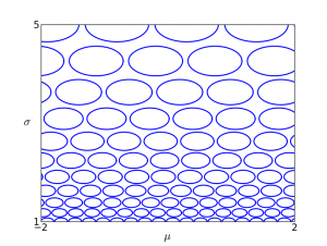
This visualization shows that when $\sigma$ is large, changing the parameters has less effect on the distribution than when $\sigma$ is small. We can also repeat this visualization for the information form representation,
\[ p(x ; h, \lambda) \propto \exp \left( -\frac{\lambda}{2} x^2 + hx \right). \]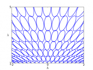
Why do the ovals fan out? Intuitively, if you rescale $h$ and $\lambda$ by the same amount, you're holding the mean fixed, so the distribution changes less than it would if you varied them independently.
Wouldn't it be great if we could find some parameterization where all the Fisher balls are unit circles? Unfortunately, there's generally no way to enforce this globally. However, we can enforce it locally by applying an affine transformation to the parameters:
\begin{align}
\eta - \eta_0 = {\bf F}_{\theta_0}^{1/2} (\theta - \theta_0). \label{eqn:trans}
\end{align}
This stretches out the parameter space in the directions of large Fisher information and shrinks it in the directions of small Fisher information. Then KL divergence looks like squared Euclidean distance near $\eta_0$:
\[ {\rm D}(\eta \| \eta_0) \approx {\rm D}(\eta_0 \| \eta) \approx \frac{1}{2} \|\eta - \eta_0\|^2. \]
What's nice about this representation is that the local properties no longer depend on the parameterization. I.e., no matter what parameterization $\theta$ you started with, the transformed space looks roughly the same near $\eta_0$, up to a rigid transformation. This gives a way of constructing mathematical objects that are invariant to the parameterization. Roughly speaking, if an algorithm is defined in terms of local properties of the model (such as gradients), you can apply the same algorithm in the transformed space, and it won't depend on the parameterization.
When we think about Fisher information in this way, it gives some useful intuitions for why it appears in so many places:
- As I mentioned above, Fisher information is most commonly motivated in terms of the asymptotic variance of a maximum likelihood estimator. I.e.,
\[ \hat{\theta} \sim {\cal N}(\theta, \frac{1}{N} {\bf F}_\theta^{-1}), \]
where $N$ is the number of data points. But what this is really saying is that if you transform the space according to (\ref{eqn:trans}), the maximum likelihood estimate is distributed as a spherical Gaussian with standard deviation $1/\sqrt{N}$. - Natural gradient [1] is a variant of stochastic gradient descent which accounts for curvature information. It basically works by stretching the space according to (\ref{eqn:trans}), and computing the gradient in the transformed space. This is analogous to Newton's method, which essentially computes the gradient in a space that's stretched according to the Hessian. Riemannian manifold HMC [2] is an MCMC sampler based on the same idea.
- The Jeffreys prior is an "uninformative" prior over the parameters of a probability distribution, defined as:
\[ p(\theta) \propto \sqrt{\det {\bf F}_\theta}. \]
Since the volume of a Fisher ball is proportional to $1/\sqrt{\det {\bf F}_\theta}$, this distribution corresponds to allocating equal mass to each of the Fisher balls. The virtue is that the prior doesn't depend on how you parameterized the distribution. - Minimum message length [3] is a framework for model selection, based on compression. From a model you construct a two-part code for a dataset: first you encode the model parameters (using some coding scheme), and then you encode the data given the parameters. If you don't want to assume anything about the process generating the data, you might choose a coding scheme which minimizes the regret: the number of extra bits you had to spend, relative to if you were given the optimal model parameters in advance. If the parameter space is compact, an approximate regret-minimizing scheme basically involves tiling the space with K Fisher balls (for some K), using log K bits to identify one of the balls, and coding the data using the parameters at the center of that ball. In the worst case, the data distribution lies at the boundary of the ball. Interestingly, this scheme has a very similar form to the Jeffreys prior, but comes from a very different motivation.
- Information geometry [4] is a branch of mathematics that uses differential geometry to study probabilistic models. The goal is to analyze spaces of probability distributions in terms of their intrinsic geometry, rather than by referring to some arbitrary parameterization. Defining a Riemannian manifold requires choosing a metric, and for a manifold of probability distributions, that metric is generally Fisher information.
[1] S. Amari. Natural gradient works efficiently in learning. Neural Computation, 1998.
[2] M. Girolami and B. Calderhead. Riemann manifold Langevin and Hamiltonian Monte Carlo methods. Journal of the Royal Statistical Society Series B, 2011.
[3] C. S. Wallace. Statistical and Inductive Inference by Minimum Message Length. Springer, 2005.
[4] S. Amari and H. Nagaoka. Methods of Information Geometry. American Mathematical Society, 2007.