Lab Progress: Laser Cutter
Ryan Adams · July 12, 2019
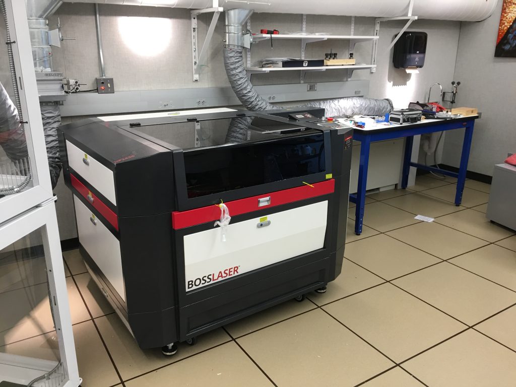
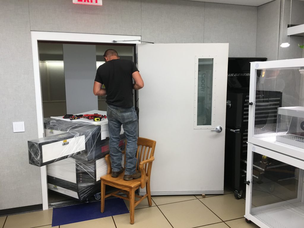
It only barely fit through the door -- required some reversible repairs to the doorframe and nearby sheetrock -- but we got it in. 150 watt Boss CO2.


Princeton University Department of Computer Science
Ryan Adams · July 12, 2019
It only barely fit through the door -- required some reversible repairs to the doorframe and nearby sheetrock -- but we got it in. 150 watt Boss CO2.
Ryan Adams · June 14, 2019
Ryan Adams · May 1, 2019
The university safety folks said we needed to have serious ventilation and fire suppression, even for consumer-grade FDM 3D-printers. The enclosures do look cool, though.
Ryan Adams · March 1, 2019
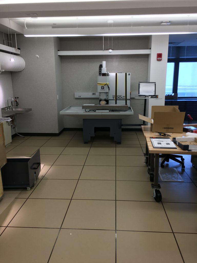
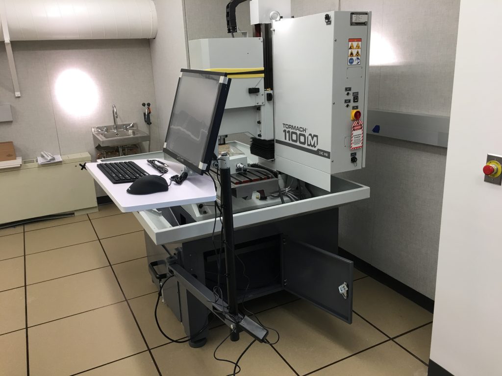
The lab is now (mostly) complete! The first piece of equipment just arrived: a Tormach 1100M. It's a bit of a toy in the machining world, but it's about the only thing that would fit in the CS building freight elevator and through the door. Even the Haas MiniMill isn't mini enough to make it to the fourth floor.


Ryan Adams · December 1, 2018
Ryan Adams · August 24, 2018
Demolition is progress, right?
Ryan Adams · July 1, 2018
After several wonderful years at Harvard, and some fun times at Twitter and Google, I've moved to Princeton. I'll miss all my amazing colleagues at Harvard and MIT, but I'm excited for the unique opportunities Princeton has to offer. I've renamed the group from the "Harvard Intelligent Probabilistic Systems" (HIPS) group to the "Laboratory for Intelligent Probabilistic Systems" (LIPS). (I should've listened to the advice of not putting the name of the university in the group name...)
I've moved all the HIPS blog posts over to this new Wordpress site, but I will keep the HIPS Github as that is where some well-known projects live, such as Autograd and Spearmint. For new projects, I've created a new repository at https://github.com/PrincetonLIPS. My new personal site is here.
Moving universities is an opportunity to explore new intellectual spaces, try new things, and take new risks. I plan to take full advantage of this and one aspect of this is that I'm going to be building a physical lab space here at Princeton. Stay tuned.
Roger Grosse · September 2, 2014
One approach to AI research is to work directly on applications that matter — say, trying to improve production systems for speech recognition or medical imaging. But most research, even in applied fields like computer vision, is done on highly simplified proxies for the real world. Progress on object recognition benchmarks — from toy-ish ones like MNIST, NORB, and Caltech101, to complex and challenging ones like ImageNet and Pascal VOC — isn’t valuable in its own right, but only insofar as it yields insights that help us design better systems for real applications.
So it’s natural to ask: which research results will generalize to new situations?
One kind of result which probably won’t generalize is: “algorithm A works better than algorithm B.” Different application areas have their own requirements. Even for a single task like object recognition, different datasets have different properties which affect how well different approaches perform. We’ve learned some things from seeing how different approaches perform in aggregate across a wide range of benchmarks; for instance, random forests are a very good general purpose classifier, and ensembles work much better than single classifiers. Benchmarks are also good for identifying talented individuals who companies should hire. But when it comes to improving our algorithms, I think it’s hard to learn very much by comparing the final performances of different approaches.
The kind of result I believe generalizes to new situations is the nature of the tradeoffs between different approaches. Consider some of what we know about neural nets and deep learning. Compared with contrastive divergence, persistent contrastive divergence gives more accurate samples, at the cost of higher variance updates. Tempered transitions is more accurate still, but much more expensive. Hessian-free optimization is better than stochastic gradient descent at accounting for curvature, but it is much harder to implement and each iteration is far more expensive. Dropout attenuates overfitting, but at the expense of higher variance in the gradients.
None of these approaches is uniformly better than its alternatives. Datasets vary a lot in factors like size, complexity, auxiliary information sources, and labeling noise which affect the tradeoffs between algorithms. For larger datasets, regularization may be less of a concern, and computation time more critical. Computational resources also make a difference, e.g. GPUs have shifted the balance in favor of dense matrix multiplies. All of these factors are likely to change between the benchmark and the practical setting, so the arg max over all the algorithmic choices is likely to change as well. (This is why Netflix never wound up using the prize-winning algorithm.) But the nature of the tradeoffs themselves seems to hold up pretty well.
Knowing the tradeoffs doesn’t give a recipe for machine learning, but it does give a strategy for designing algorithms. Researchers have generally worked on several problems or datasets, and we know which algorithms work well and which factors are important on these datasets. Using these as reference points, we think about how the new problem differs (is it larger? noisier?), and that tells us in which directions to adjust. From this starting point, we can run diagnostics to tell us which issues are hurting performance and what useful sources of information are our methods overlooking, and this will inform our choice of algorithms.
This is part of why companies are spending so much money to hire top machine learning researchers. Quite a lot is known about machine learning, but the knowledge is still highly context dependent. (It’s a good thing for us researchers that “A is better than B” results don’t generalize; otherwise, there would be One Algorithm to Rule them All, and little room for new insight.)
It may seem obvious that if we can’t replicate the real world in our benchmarks, we should at least try to get as close as possible. Shouldn’t we be working with large image datasets as representative as possible of the distribution of all images? Shouldn’t we build the very best performing algorithms that we can on these problems, so that they will be close to what’s used in practice? The problem is, the larger the dataset and the more complex the algorithm, the harder it is do to science.
Brian Kernighan once said, “Everyone knows that debugging is twice as hard as writing a program in the first place. So if you’re as clever as you can be when you write it, how will you ever debug it?” But running careful and meaningful experiments is harder still than debugging. You need to vary a lot of factors and measure their effect, which requires running the algorithm many more times than if you simply wanted to use it. Controlling for confounding factors requires a clear understanding of how everything fits together. If your algorithm is at the frontier of what you can implement, or of what can be run on modern computing technology, then how will you ever run experiments with it?
Trying to bust the hardest benchmarks usually pushes us to the frontier of what our brains and our computers can handle. This reflects itself in the sorts of experiments we run. If you look through recent deep learning or Bayesian nonparametrics papers which use toy datasets, you’ll find carefully controlled experiments which vary one factor and show that this makes a difference. Authors are expected not just to show that their method works better, but also to present evidence for why it works better. But with the most challenging benchmarks, authors typically compare their final performance against numbers previously published in the literature. These numbers were obtained using a completely different system, and it’s often hard to understand the reason for the improvement.
I briefly worked on an object detection project with Joseph Lim, using the Pascal VOC dataset. Like most people working on object detection at the time, we built on top of Pedro Felzenswalb’s deformable part model software package. For reasons I won’t go into, we tried replacing the SVM package it used with a different SVM package, and this led to a huge drop in performance. This seemed nonsensical — both packages were optimizing the same convex objective, so shouldn’t they be interchangeable? After a week of digging (these models take a long time to run), Joseph figured out that it had to do with a difference in the stopping criterion. But if such subtle implementation details can have such a big impact overall, what are we to make of performance comparisons between completely different systems implemented by different individuals?
As I argued above, if we want results which will generalize, we need a clear causal explanation for why one algorithm behaves differently from another. With large datasets where experiments take days or weeks, complex algorithms that require building on someone else’s code, and time pressure to beat everyone else’s numbers, there just isn’t enough time to run enough experiments to get a full understanding. With small datasets, it’s possible to chase down all the subtle issues and explain why things happen.
In recent years, neural nets have smashed lots of benchmarks, but it’s important to remember that this follows upon decades of empirical sleuthing on toy datasets. In fact, the toy datasets are still relevant: even in the Big Data Capital of the World, Geoff Hinton still runs experiments on MNIST. I think these datasets will continue to deliver insights for some time to come.
Roger Grosse · August 26, 2013
When we talk about priors and regularization, we often motivate them in terms of "incorporating knowledge" or "preventing overfitting." In a sense, the two are equivalent: any prior or regularizer must favor certain explanations relative to others, so favoring one explanation is equivalent to punishing others. But I'll argue that these are two very different phenomena, and it's useful to know which one is going on.
The first lecture of every machine learning class has to include a cartoon like the following to explain overfitting: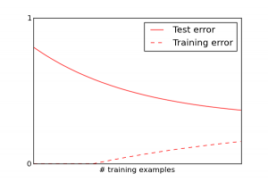
This is more or less what happens if you are using a good and well-tuned learning algorithm. Algorithms can have particular pathologies that completely distort this picture, though.
Consider the example of linear regression without a regularization term. I generated synthetic data with $D = 100$ feature dimensions, with everything drawn from Gaussian priors. Recall that the solution is given by the pseudoinverse formula $X^\dagger y$, i.e. from the set of points which minimize error on the training set, it chooses the one with the smallest norm. Here's what actually happens to the training and test error as a function of the number of training examples $N$ (the dotted line shows Bayes error):
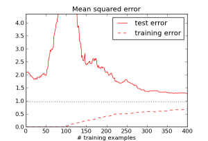
Weird -- the test error actually increases until $N$ roughly equals $D$. What's going on?
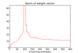
When $N \ll D$, it's really easy to match all the training examples. E.g., when N = 1, there's a $D-1$ dimensional affine space which does this. But as $N$ becomes closer to $D$, it gets much harder to match the training examples, and the algorithm goes crazy trying to do it. We can see this by looking at the norm of the weight vector $w$:
So really, the large error is caused by the algorithm doing something silly: choosing a really large weight vector in order to match every training example. Now let's see what happens when we add an L2 regularization term $\lambda \|w\|^2$. Here are the results for several different choices of lambda:
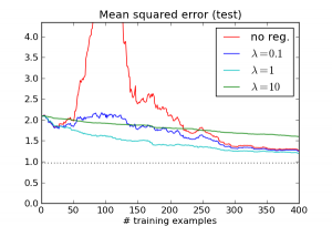
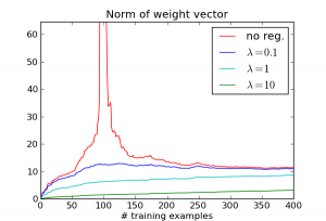
The effect disappears! While the different $\lambda$ values occupy different points on the overfitting/underfitting tradeoff curve, they all address the basic issue: the regression algorithm no longer compulsively tries to match every example.
You might ask, doesn't this regularizer encode information about the solution, namely that it is likely to be near zero? To see that the regularization term really isn't about this kind of knowledge, let's concoct a regularizer based on misinformation. Specifically, we'll use an L2 regularization term just as before, but instead of centering it at zero, let's center it at $-w$, the exact opposite of the correct weight vector! Here's what happens:
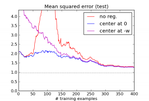
This is indeed a lousy regularizer, and for small training set sizes, it does worse than having no regularizer at all. But notice that it's still enough to eliminate the pathology around $N=D$, and it continues to outperform the unregularized version after that point.
Based on this, I would argue that for linear regression, L2 regularization isn't encoding knowledge about where good solutions are likely to be found. It's encoding knowledge about how the algorithm tends to misbehave when left to its own devices.
Usually, priors and regularizers are motivated by what they encourage rather than what they prevent, i.e. they "encourage smoothness" or "encourage sparsity." One interesting exception is Hinton et al.'s paper which introduced the dropout trick. Consider the title: "Improving neural networks by preventing co-adaptation of feature detectors." Co-adaptation refers to a situation where two units representing highly correlated features wind up with opposing weights. Their contributions wind up mostly canceling, but the difference may still help the network fit the training set better. This situation is unstable, because the pair of units can wind up behaving very differently if the data distribution changes slightly. The dropout trick is to randomly turn off 50% of the units on any given iteration. This prevents co-adaptation from happening by making it impossible for any two units to reliably communicate opposite signals.
Next time you try to design a prior or regularizer, think about which you're doing: are you trying to incorporate prior knowledge about the solution, or are you trying to correct for the algorithm's pathologies?
David Duvenaud · August 1, 2013
In this post, I'll summarize one of my favorite papers from ICML 2013: Fast Dropout Training, by Sida Wang and Christopher Manning. This paper derives an analytic approximation to dropout, a randomized regularization method recently proposed for training deep nets that has allowed big improvements in predictive accuracy. Their approximation gives a roughly 10-times speedup under certain conditions. Much more interestingly, the authors also show strong connections to existing regularization methods, shedding light on why dropout works so well.
The idea behind dropout is very simple: during each evaluation of the neural net during training, half the inputs and hidden units are randomly 'dropped' (set to zero). This simple technique allowed large improvements in predictive accuracy for deep nets. However, it was not immediately clear why it works so well. The original paper gives several intuitions about why dropout works. One proposed explanation is that individual hidden units are discouraged from developing complex (and possibly brittle) dependencies on each other. We'll return to that question later.
The key insight in the fast dropout paper is this: If the input to each node in a neural network is a weighted sum of its inputs - and if some of those inputs are randomly being set to zero, then the total input is actually a weighted sum of Bernoulli random variables. By the Central Limit Theorem, this sum can be well-approximated by a Gaussian when a neuron has many inputs with comparable variance. The authors derive the mean and variance of these Gaussians, and can then approximately integrate over all exponentially-many combinations of dropouts in a one-layer network. They also approximate the output of each neuron with a Gaussian, by locally-linearizing the nonlinearity in each neuron, and derive deterministic update rules for the multi-layer case. This trick leads to a roughly 10-times speedup in training times. More interesting than the speedup, though, is that this approximate dropout technique is equivalent in some ways to standard approaches.
The first equivalence shown is: if you normalize your data features to all have the same variance, then ridge regression is exactly equivalent to least-squares linear regression using dropout! This means that dropout is a regularization technique that's invariant to rescaling of the inputs, which may be one reason why it works so well. In deep nets, this may be especially helpful, since the scale of the hidden node activations may change during training.
The second equivalence shown is that a one-layer neural network trained using dropout is approximately optimizing a lower bound on the model evidence of a logistic regression model. This result suggests that dropout is closely related to expectation-maximization (or, more generally, variational Bayes). The original dropout paper mentions a similar result - for one-layer networks, dropout approximately optimizes the geometric mean of the likelihood of all possible ways of removing nodes from the network - but the explicit derivations in the fast dropout paper make the link much clearer.
So, this paper gives us two new ways to think about dropout - as a scale-invariant regularizer, and as an approximate variational method. The success of dropout suggests that, even for large datasets, regularization of deep nets is still very important. Perhaps we should take a second look at variational inference in deep Bayesian neural networks, or further investigate scale-invariant regularization methods.
Thanks to Oren Rippel and Roger Grosse for helpful comments.
Update: Kevin Swersky pointed out a follow-up paper with even more connections: Dropout Training as Adaptive Regularization