Say you have a set of $n$ $p$-dimensional iid samples $$\{ \textbf x_i \}_{i=1}^n$$ drawn from some unknown continuous distribution that you want to estimate with an undirected graphical model. You can sometimes get away with assuming the $\textbf x_i$'s are drawn from a multivariate normal (MVN), and from there you can use a host of methods for estimating the covariance matrix $\Sigma$, and thus the graph structure $\Omega = \Sigma^{-1}$ (perhaps imposing sparsity constraints for inferring structure in high dimensional data, $n<<p$).
In other cases the Gaussian assumption is too restrictive (e.g. when marginals exhibit multimodal behavior).
One way to augment the expressivity of the MVN while maintaining some of the desirable properties is to assume that some function of the data is MVN. So instead of modeling the $\textbf x_i$'s as MVN, relax the assumption and model a function of the components $f(\textbf x_i) = (f_1(x_1), ..., f_p(x_p))$ as MVN with mean $\mu$ and covariance $\Sigma$. Now the goal is to estimate $f, \mu, \Sigma$, which characterizes the distribution. Distributions of this type are referred to as nonparanormal (or Gaussian copula distribution).
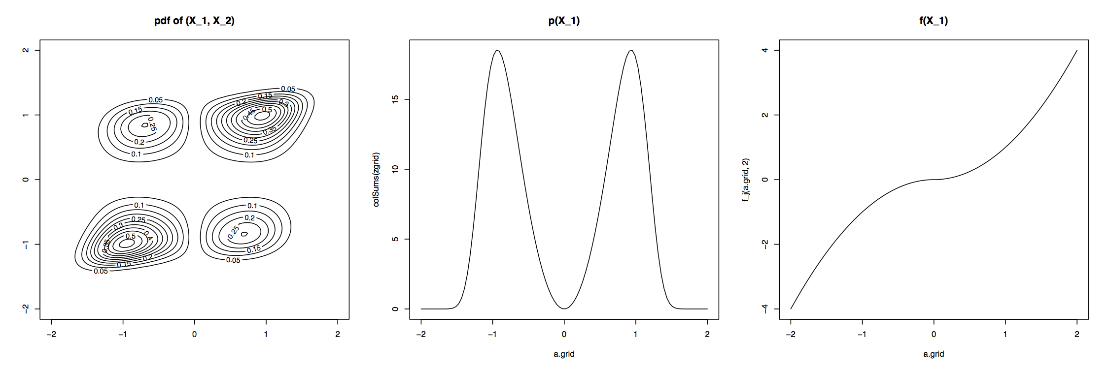
The plots below show an example $NPN$ with $f_j(x_j) = sgn(x_j)|x_j|^{\alpha_j}$. The plots show the contours for a 2-D $NPN$ distribution, one of the marginals, and one of the transformation functions $f$ (recreated from Lui 2009).

More formally, $X=(X_1, ..., X_p)^T$ has a nonparanormal distribution if there exist a set of functions $\{f_1, ..., f_p\}$ such that $(f_1(X_1), ..., f_p(X_p)) \sim N(\mu, \Sigma)$. This is denoted by $X \sim NPN(\mu, \Sigma, f)$ (Lui 2009).
The resulting density function of the $NPN(\mu, \Sigma, f)$ (assuming the $f$'s are continuous and monotonic) is:
$$ p(x) = \frac{1}{(2\pi)^{p/2}|\Sigma|^{1/2}} \exp \left( -\frac{1}{2}(f(x)-\mu)^T \Sigma^{-1} (f(x) - \mu) \right) \prod_{i=1}^p |f_j'(x_j)| $$
From here, you can derive the important property that if $X\sim NPN(\mu, \Sigma, f)$ is nonparanormal and each $f_i$ is differentiable, then the conditional independence structure of the data is still encoded in the inverse covariance matrix $\Omega = \Sigma^{-1}$. It also follows that the graph structure (i.e. the inverse covariance zero locations) of the transformed, normal variables is identical to the graph structure of the non normal variables. This allows you to estimate the graph structure as if the data were normal (with some care).
Now a whole bunch of techniques (graph/structure estimation, inference, etc) can be extended to this richer set of models. Lui et al 2009 present techniques for estimating undirected graphical models when $n << p$. A recent paper from NIPS (Elidan and Cario) formalizes belief propagation in a nonparanormal setting.
Another interesting study of inverse covariance and graph structure (on discrete data) is the "No Voodoo Here" (Loh and Wainwright) paper from NIPS this past year. Though I haven't closely read it, a close examination of the two may shed light on new structure estimation algorithms in high dimensional data.
