
I don't have a favorite distribution, but if I had to pick one, I'd say the gamma. Why not the Gaussian? Because everyone loves the Gaussian! But when you want a prior distribution for the mean of your Poisson, or the variance of your Normal, who's there to pick up the mess when the Gaussian lets you down? The gamma. When you're trying to actually sample that Dirichlet that makes such a nice prior distribution for categorical distributions over your favorite distribution (how about that tongue twister), who's there to help you? You guessed it, the gamma. But if you want a distribution that you can sample millions of times during each iteration of your MCMC algorithm, well, now the Gaussian is looking pretty good, but let's not give up hope on the gamma just yet.
This situation might arise if you are Gibbs sampling a large graphical model in which many nodes are conditionally independent and conjugate with a gamma, beta, or Dirichlet prior. Deep belief networks come to mind. We often see Gaussians used in this scenario, partly because uniform r.v.'s can be efficiently transformed into Gaussian r.v.'s by the Box-Muller method or Marsaglia's Ziggurat algorithm [1]. Unfortunately there is no analytic method of transforming uniform r.v.'s into gamma samples (without the computationally expensive evaluation of the inverse CDF). Instead, Matlab and Numpy use rejection sampling to generate gammas.
For those interested in GPU-based parallel sampling implementations, the inherent unpredictability of the number of rejections poses a problem since GPUs are much more efficient when all threads operate in lock-step and the number of iterations is predetermined. Hence libraries like cuRAND and do not ship with a gamma generator. A naive solution is to place a limit on the number of allowed rejections and run each thread the worst-case number of iterations. For this post I wrote a simple CUDA kernel that implements this naive solution and compared its performance against that of Matlab's gamrnd() and Numpy's random.gamma() functions. The code is available here.
Before jumping into the results, let's consider the rejection sampling approaches used by Matlab and Numpy. Both use the Mersenne Twister [2] as the default pseudorandom number generator (PRNG) [3]. Both also use Marsaglia and Tsang's simple rejection sampling algorithm[4] to transform one uniform r.v. and one standard normal r.v. into a single gamma r.v., though the generation of the standard normal r.v.'s differs. Whereas Matlab uses the Ziggurat method [1], Numpy uses a modification of the Box-Muller method which avoids trigonometric functions, also due to Marsaglia [5,6].
Marsaglia and Tsang's gamma algorithm is pretty neat. The idea is to take a r.v. with a nearly Gaussian density and transform such that the resulting r.v. has a gamma density. Then we can use rejection sampling with a Gaussian proposal distribution, and transform to get a gamma. To maintain computational efficiency, the calculation of the inverse transformation must be fairly simple; in particular, we would like to avoid transcendental functions (eg. exp, log, sin) and stick to algebraic manipulations like multiplication, small powers, and, sparingly, division and square roots [7]. They choose the transformation $h(x)=d(1+cx)^3$ for $-1/c<x<\infty$ and $\alpha>1$, which yields a density proportional to
\begin{equation}
p(x)\propto e^{(k\alpha-1)\ln(1+cx)-d(1+cx)^{k}+d} \leq e^{-\frac{1}{2}x^{2}}.
\end{equation}
Letting $k=3$, $d=\alpha-1/k$, $c=1/\sqrt{k^2 \alpha -k}$, and taking their word that the normalization constants cancel, determining whether a uniform r.v. $u$ is less than the ratio $p(x)/\mathcal{N}(x\,|\,0,1)$ is equivalent to testing
\begin{equation}
\ln(u)<\frac{1}{2}x^{2}+d-dv+d\ln(v).
\end{equation}
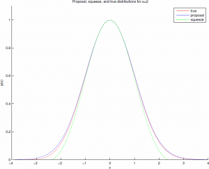
This comparison can be made more efficient with the "squeeze" $s(x)=(1-0.0331x^4)e^{-\frac{1}{2}x^{2}}\leq p(x)\leq e^{-\frac{1}{2}x^{2}}$, with an easily computable acceptance ratio, such that there is low probability of the squeeze being rejected when the true sample should be accepted. For $\alpha=2$ the acceptance ratio is about 98.1%. These distributions are shown graphically below.
So at this point you might be thinking, "Scott, why are we worrying about a couple logs? This is 2013." That is a fair point -- if you're only sampling a handful of gammas at a time then it really doesn't matter. But if you're generating billions, as you might in a large graphical model or a deep belief network, and especially if you're implementing this on a GPU, the cost of those functions can add up quickly.
With this in mind, I implemented the Marsaglia-Tsang algorithm in a CUDA kernel along with a simple PyCuda script to test different parameter settings and copy the result to the host. The CUDA kernel takes in $M$ normal and uniform random variables for each of the $N$ gammas it generates, and runs $MN$ threads in parallel. Each thread generates a proposed gamma r.v. and checks whether or not it is acceptable. Then a second kernel runs a log-time reduction to choose, for each of the $N$ samples, the first acceptable gamma from its $M$ proposals. If all proposals are rejected (probability $\approx (1-.98)^M$) we return an error. The uniform and standard normal r.v.'s are generated with the cuRAND library's XORWOW PRNG, which is lighter weight than the Mersenne Twister. The average run time to sample a batch of gammas (with randomly chosen parameters) as a function of batch size is shown below.
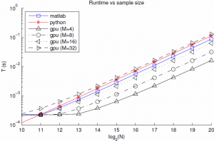
Of note, for $M=8$ the GPU implementation is about 2.5x faster than Matlab, and suffers from only about 10e-7 failure rate. I suspect that the flat part of the curve for $N=10\ldots 13$ is partly due to timer precision, and partly to fixed costs of GPU calls and copies. Finally, and most importantly, the sample time still scales linearly with the batch size. If we look into the breakdown of the GPU time we see that this is due to linear scaling of both the PRNG, as expected due to its sequential nature, but also due to the kernel time. This is rather surprising since the threads are nearly independent, and suggests that the cost of each GPU call is proportional to the grid size. For these $M$, the affects of the log-time reduction are negligible.
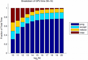
Since the PRNG is the dominating component, it makes sense to start looking for improvements there. CuRand supports parallel PRNG's, but the generation of pseudorandom numbers is still inherently serial so we will only save a constant factor. Nevertheless, the gain from 10 or 100 independent PRNGs would be significant for large batch sizes. Finally, for many GPU applications, the availability of native gamma sampling algorithms is very convenient and faster than copying from the host. I have made use of this code in some of my own MCMC applications, and hope you might find it useful as well.
All code is available at https://bitbucket.org/swl28
[1] George Marsaglia and Wai Wan Tsang. "The Ziggurat Method for Generating Random Variables". Journal of Statistical Software 5 (8). (2000)
[2] M. Matsumoto and T. Nishimura, "Mersenne Twister: A 623-dimensionally equidistributed uniform pseudorandom number generator", ACM Trans. on Modeling and Computer Simulation. Vol. 8, No. 1, January pp.3-30 (1998).
[3] To check this call RandStream.getGlobalStream() in Matlabor numpy.random.get_state() in Python. Both should return "mt19937" by default.
[4] George Marsaglia and Wai Wan Tsang. "A simple method for generating gamma variables." ACM Trans. on Mathematical Software. Volume 26, No. 3, September pp. 363-372 (2000).
[5] You can check out the numpy source here and here
[6] In case you haven't noticed, Marsaglia was a computational statistics rock star.
[7] As an aside, the computation of transcendental functions depends upon your architecture. Typical approximation methods use tables in conjunction with Taylor series approximations or Chebyshev polynomials. The computation of square roots has an ancient history; to the best of my knowledge the binary digit-by-digit method and the Babylonian method are viable, but well-tuned Newton-Raphson is common for sqrt and division.