
Annealed importance sampling [1] is a widely used algorithm for inference in probabilistic models, as well as computing partition functions. I'm not going to talk about AIS itself here, but rather one aspect of it: geometric means of probability distributions, and how they (mis-)behave.
When we use AIS, we have some (unnormalized) probability distribution $p(x)$ we're interested in sampling from, such as the posterior of a probabilistic model given observations. We also have a distribution $q(x)$ which is easy to sample from, such as the prior. We need to choose a sequence of unnormalized distributions $f_t(x)$ indexed a continuous parameter $t \in [0, 1]$ which smoothly interpolate between $q$ and $p$. (I use $f_t$ because later on, $p$ and $q$ will correspond to directed graphical models, but the intermediate distributions will not.)
A common choice is to take a weighted geometric mean of the two distributions. That is, $f_t(x) = q(x)^{1-t} p(x)^t$. This is motivated by examples like the following, where we gradually "anneal" from a uniform distribution to a multimodal one.
This is the desired behavior: the intermediate distributions look like something in between $p$ and $q$.
However, most of the probabilistic models we work with include latent variables $u$ in addition to $x$, and the distribution $p(x)$ is defined implicitly in terms of the integral $p(x) = \int p(u, x) du$. In these cases, computing the geometric mean as we did above can be intractable, since it requires summing/integrating out the latent variables. Another approach would be to take the geometric mean of the full joint distribution over $x$ and $u$. However, this geometric mean might not even be defined, if the dimensionality of $u$ in the two models is different.
Instead, we often use the following "doubling" trick introduced by [2]. We introduce an expanded state space which includes two sets of latent variables $u_1$ and $u_2$. We can view $q$ as a distribution $q(u_1, u_2, x)$ over the expanded state space where $x$ depends only on $u_1$, and hence $u_2$ is irrelevant to the model. Similarly, $p$ defines a distribution on this space where $x$ depends only on $u_2$. Then it makes mathematical sense to take the geometric mean in this expanded space.
For instance, suppose $q$ and $p$ both define directed graphical models, i.e. they are defined in terms of a factorization $q(u, x) = q(u) q(x | u)$. For simplicity, assume nothing is observed. Then the intermediate distributions would take the following form:
$f_t(u_1, u_2, x) = q(u_1) p(u_2) q(x | u_1)^{1-t} p(x | u_2)^t.$
Intuitively, $u_1$ and $u_2$ are both drawn from their corresponding priors in each distribution, and we gradually reduce the coupling between $x$ and $u_1$, and increase the coupling between $x$ and $u_2$.
Consider the following model, where ${\bf u}$ and ${\bf x}$ are vectors in ${\mathbb R}^D$:
\[\begin{align*} p({\bf u}) = q({\bf u}) &= {\cal N}({\bf u} | {\bf 0}, r{\bf I}) \\ p({\bf x} | {\bf u}) = q({\bf x} | {\bf u}) &= {\cal N}({\bf x} | {\bf u}, (1 - r) {\bf I}). \end{align*}\]In this model, ${\bf x}$ is always distributed as ${\cal N}({\bf 0}, {\bf I})$, and it is coupled with the latent variable ${\bf u}$ to an extent that depends on the coupling parameter $r$. The two models $p$ and $q$ happen to be identical. This is a toy example, but the problem it will illustrate is something I've run into in practice.
We might expect that when we take the geometric mean of these distributions, we get the same distribution, or at least something close. Not so. For instance, the latent variables $u_1$ and $u_2$ are independent under either $p$ or $q$, since both are directed models with no evidence. In the univariate case ($D=1$), here is the joint distribution of $u_1$ and $u_2$: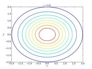
Counterintuitively, when we take the geometric mean ($t=1/2$), the two variables become coupled: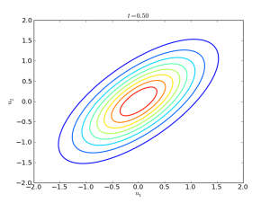
What's going on? The following figure shows what happens when we take the geometric mean (shown in red) of $q(x|u_1)$ and $p(x|u_2)$, with $u_1 = -0.5$ and $u_2 = 0.5$: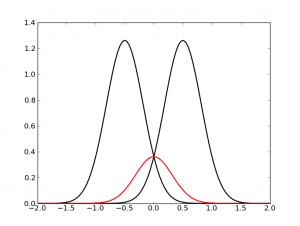
Essentially, when two distributions disagree with each other, their geometric mean is small everywhere. This means less probability mass is allocated to regions where $u_1$ and $u_2$ are much different. Therefore, the geometric mean causes $u_1$ and $u_2$ to become positively correlated.
Now let's make the model a bit more complicated by adding the coupling parameter $r$ as a random variable. Let's give it a uniform prior. Under $p$ and $q$, the distribution over $r$ is uniform, since they are directed models with no evidence.
However, under the geometric mean distribution $f_{1/2}$, the marginal distribution over $r$ is very much non-uniform: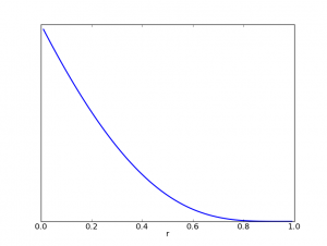
(In this figure, I used $D=10$.) When the coupling parameter is large, $u_1$ and $u_2$ are required to agree with each other, whereas when $r$ is small, it doesn't matter. Therefore, the distribution strongly "prefers" explanations which involve the latent variables as little as possible.
In general, geometric means of two complex distributions can have properties very different from either distribution individually. This can lead to strange behaviors that make you suspect there's a bug in your sampler. I don't know of any good alternative to the approach given above, but don't be surprised if geometric means don't always do what you expect.
[1] Radford Neal. Annealed Importance Sampling. Statistics and Computing, 2001.
[2] Ruslan Salakhutdinov and Iain Murray. On the quantitative analysis of deep belief networks. ICML 2008.